Isolated Block Stability Method

Introduction

The isolated block stability method is based on an academic code developed at Mines Paris Tech (Ghazal et al. (2011a), Ghazal (2013), Ghazal et al. (2011b). The linear version is now implemented in 3DEC and can be applied using a simple command line. The method evaluates the stability of a single 3D rigid block of any shape located at the surface of an underground excavation. The block is “isolated”, meaning it is analyzed as if it exists alone in the rock mass, that is, the presence of other potential blocks is ignored. The block moves as a rigid body in translation and rotation and interacts with the surrounding continuous rock mass via joint elements. The block is initially, before excavation, subjected to initial stresses applied on all of its faces. The approach consists of calculating the block movement and stress variation on faces due to the excavation process (the release of stresses on the excavation faces).

Theoretically, the method gives the same solution as an equivalent 3DEC simulation of an excavation with only one block located at the free surface, considering the “rigid blocks” hypothesis. However, it is more straightforward: only the block geometry, joint properties and stress data are needed.

The method is an interesting alternative to block stability methods based on the limit equilibrium approach and “keyblock” theory (Goodman and Shi (1985), Warburton (1985)). Comparisons to such approaches are detailed in Ghazal et al. (2011a) and Ghazal (2013).

The method was developed for elastic as well as elasto-plastic joints with a Mohr-Coulomb failure criterion and dilation. However, the current implementation in 3DEC considers only elastic joints. The stability is thus evaluated by calculating a factor of safety on the block faces.

Description of the Method

Approach

Consider a rigid block located at the surface of an underground excavation. In the initial state, before excavation, block faces are subjected to in situ stress. The excavation process consists of releasing the stresses applied on the future free face. This triggers a variation of stresses on other faces to keep the block at equilibrium. The variation of stresses is controlled by joint constitutive laws. Additionally, rigid body block movement relates the displacement at each point of the faces to a displacement and rotation at the center of the block.

By solving the equilibrium equations between the initial state prior to excavation and the final state after excavation when stresses at the free face are released — and considering the block movement as a rigid body and joint constitutive laws — it is possible to build a linear system where the only unknowns are the block translation and rotation.

Figure 1: Conceptual scheme of block stability code.

Equations

Block Equilibrium

Block equilibrium (forces and moments) is written in variational terms for a relaxation rate \(d \lambda\) applied to the resultants of forces and moments (\(\mathbf{F}_0\) and \(\mathbf{M}_0\)) acting on the free face before excavation.

(1)\[\int_{\Sigma_J}d \pmb{σ}\ dS+d\lambda\ {\mathbf{F}}_0=\mathbf{0}\]

(2)\[\int_{\Sigma_J}\mathbf{x}\times d\pmb{σ}\ dS+d\lambda\ {\mathbf{M}}_0=\mathbf{0}\]

where

\({\mathbf{F}}_0\) and \({\mathbf{M}}_0\) are the opposite of the resultant force and moment vectors acting on the free block surfaces \(\Sigma_L\) before excavation;

\(\pmb{σ}\) is the stress vector acting on a point \(\mathbf{x}\) of the joint faces \(\Sigma_J\), the origin being a fixed point located inside the block; and

\(\lambda\) represents the “deconfining” or stress relaxation factor.

When dealing with a linear elastic system these two equations can be simplified

(3)\[\int_{\Sigma_J}\mathrm{\Delta} \pmb{σ}\ dS+{\mathbf{F}}_0=\mathbf{0}\]

(4)\[\int_{\Sigma_J}\mathbf{x}\times\mathrm{\Delta}\pmb{σ}\ dS+\ {\mathbf{M}}_0=\mathbf{0}\]

Block Movement as a Rigid Body

The block displacement at every point can be related to the block displacement at the center and block rotation, considering the hypothesis of small rotations.

(5)\[d\mathbf{u}=d\mathbf{U}+d\mathbf{W}\times\mathbf{x}\]

where

\(\mathbf{U}\) is the displacement vector at the block’s centroid (or any other point inside the block)

\(\mathbf{W}\) the rotation vector of the block; and

\(\mathbf{u}\) is the displacement at a given point \(\mathbf{x}\) of the block.

Figure 2: Block movement as a rigid body in translation and rotation (from Ghazal (2013)).

Joint Constitutive Equations

A linear behavior in the normal and shear direction is given by Equations (6) and (7):

(6)\[d\sigma_n=-k_n\ du_n\]

(7)\[d{\mathbf{\sigma}}_t=-k_s\ d{\mathbf{u}}_t\]

where at a given point of the joint (block faces),

\(u_n\) is the normal displacement;

\(\sigma_n\) is the normal stress;

\(k_n\) is the normal stiffness;

\({\mathbf{u}}_t\) is the shear displacement vector;

\({\mathbf{\sigma}}_t\) is the shear stress vector; and

\(k_s\) is the shear stiffness.

By recognizing that \(d\pmb{σ}=d\sigma_n\mathbf{n}+d\pmb{σ}_t\) , \(du_n=\ d\mathbf{u}.\mathbf{n}\) and \(d{\mathbf{u}}_t=d\mathbf{u}-(d\mathbf{u}.\mathbf{n})\mathbf{n}\) , Equations (6) and (7) can be combined into the following equation

(8)\[d\pmb{σ}=-\underline{\underline{K}}\ d\mathbf{u}\]

\[\underline{\underline{K}}=k_t\underline{\underline{I}}+(k_n-k_s)\ \mathbf{n}\ \otimes\ \mathbf{n}\]

where

\(\underline{\underline{I}}\) is the identity matrix;

\(\mathbf{n}\) represents the exterior normal to the block face at a given point; and

\(\mathbf{n}\ \otimes\ \mathbf{n}=\mathbf{n}\ {\mathbf{n}}^T\) is the symmetric tensor \(n_i\ n_j\).

Note that the sign convention assumes normal stress is negative in compression and \(du_n>0\) denotes that the block is approaching the rock mass.

In the most advanced version of this method, the joint is assigned a hyperbolic behavior in the normal direction with a maximum closure. In the shear direction the behavior is elasto-plastic with Coulomb yield criterion and dilation during the plastic phase. However, the current 3DEC implementation considers only elastic linear behavior in the normal and shear directions. Nonlinear behavior could also be implemented in 3DEC in the future.

Linear System

Solving the equations above between the initial state before excavation and the final state after excavation (Equations (3), (4), (5), (6), and (7)) leads to the following linear system:

(9)\[\begin{split}\underline{\underline{R}}\left[\begin{matrix}\mathbf{U}\\\mathbf{W}\\\end{matrix}\right]=\left[\begin{matrix}{\mathbf{F}}_0\\{\mathbf{M}}_0\\\end{matrix}\right]\end{split}\]

(10)\[\begin{split}\underline{\underline{R}}=\left[\begin{matrix}\underline{\underline{A}}&\underline{\underline{B}}\\\underline{\underline{D}}&\underline{\underline{C}}\\\end{matrix}\right]\end{split}\]

where

\(\underline{\underline{A}}\ \underline{\underline{B}}\ \underline{\underline{C}}\ \underline{\underline{D}}\) represent integrations on the joint surfaces \(\Sigma_J\) of matrix \(\underline{\underline{K}}\) (generalized elastic joint stiffness matrix \(d\pmb{σ}=-\underline{\underline{K}}\ d\mathbf{u}\) ) :

(11)\[\underline{\underline{A}}=\int_{\Sigma_J}{\underline{\underline{K}}\ dS}\ \ \ \ \ \ \ \ \underline{\underline{B}}=\int_{\Sigma_J}{\underline{\underline{K}}\ \underline{\underline{r}}\ dS}\]

(12)\[\underline{\underline{C}}=\int_{\Sigma_J}{{\underline{\underline{r}}}^T\ \underline{\underline{K}}\ \underline{\underline{r}}\ dS}\ \ \ \ \ \ \ \ \underline{\underline{D}}=\int_{\Sigma_J}{{\underline{\underline{r}}}^T\ \underline{\underline{K}}\ \ dS}\]

\(\underline{\underline{r}}\) is the rotation vector of the position vector \(\mathbf{x}\) (the origin is a fixed reference point located inside the block) defined such as for any vector \(\mathbf{a}\), \(\underline{\underline{r}}\ \mathbf{a}=\ \mathbf{a}\times\mathbf{x}\)

If \(\mathbf{x}=\left[x_1\ \ x_2\ \ x_3\right]^T\ \ \ \ \ ,\ \ \ \ \ \underline{\underline{r}}=\left[\begin{matrix}0&x_3&-x_2\\-x_3&0&x_1\\x_2&-x_1&0\\\end{matrix}\right]\)

Surface integration is done using face discretization (the block faces are introduced as surface meshes).

Stability evaluation

After solving the linear system (Equation (9)), the displacement (Equation (5)) and stress state (Equations (6) and (7)) at every point of the block can be evaluated.

Then a safety factor is calculated at every mesh of the block faces by:

(13)\[\begin{split}FOS = \begin{cases} \dfrac{-\sigma_n \tan\phi + c}{||\pmb{σ}t||} & \text{ if } \sigma_n \leq 0 \\ \hspace{12mm} 0 & \text{ if } \sigma_n > 0 \end{cases}\end{split}\]

A single safety factor per block may be obtained in two ways: either consider the minimum safety factor on all block faces, or compute the mean safety factor from \(FOS_{mean}=\sum{FOS_i\ A_i/\sum A_i}\) (where \(A_i\) is the area of face \(i\)).

Example Applications

Single Block Stability

The isolated block stability method is applied to a single tetrahedral block. The block is located at the roof of a cylindrical excavation of radius R = 5 m, at a depth of 200 m, with a rock mass density \(\rho\) = 2500 kg/m³. The block is the maximum volume block constituted by the intersection of three joints with the roof of the excavation (dip directions 0°, 120°, and 240°, all having the same dip 60°). Joint strength properties are set to \(\phi\) =35° and \(c\) = 0 MPa for the calculation of the factor of safety.

This model demonstrates the advantage of this method. The boundaries of the tunnel need not be placed very far from the excavation because only the block geometries and in situ stresses influence the result. The model geometry is shown in Figure 3.

The factors of safety (FOS) for the block faces are calculated using the command block analyze-stability for \(K_0\) = 1 and \(k_n/k_s\) = 10. After the calculation is complete, a list of blocks and their minimum and mean FOS are printed to the screen. Note that joined blocks are considered a single block in this analysis and the leader ID is given. Each block is also assigned a group name equal to the leader ID in the slot “isolated_block.”

Note also that joined faces are assigned a group name “internal_face” in the “Default” group slot. FOS is not calculated on these faces.

Block faces and contours are plotted using Kinematic FOS (set plotting “Contour” on a Face plot item; pull “Kinematic FOS” from the “Contour” attribute pulldown). The range can be used to plot only the faces with a group name equal to the leader ID of the block with the minimum FOS (in this case, 128). Figure 4 shows the distribution of FOS on the faces of the wedge block.

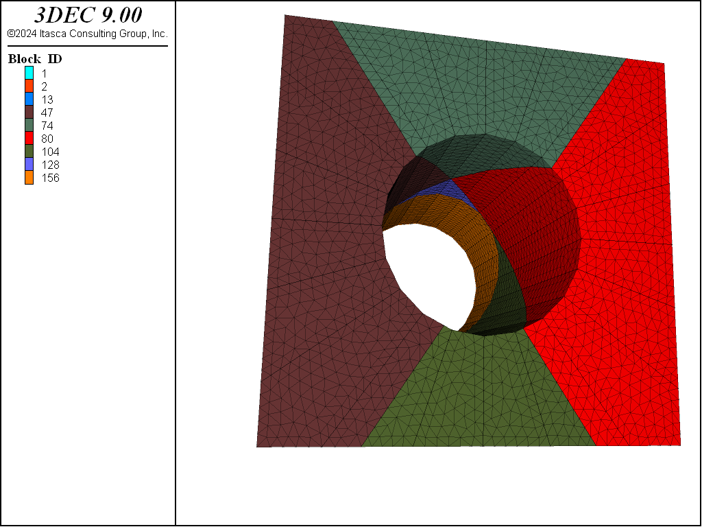
Figure 3: Tunnel model used in the kinematic FOS calculation.

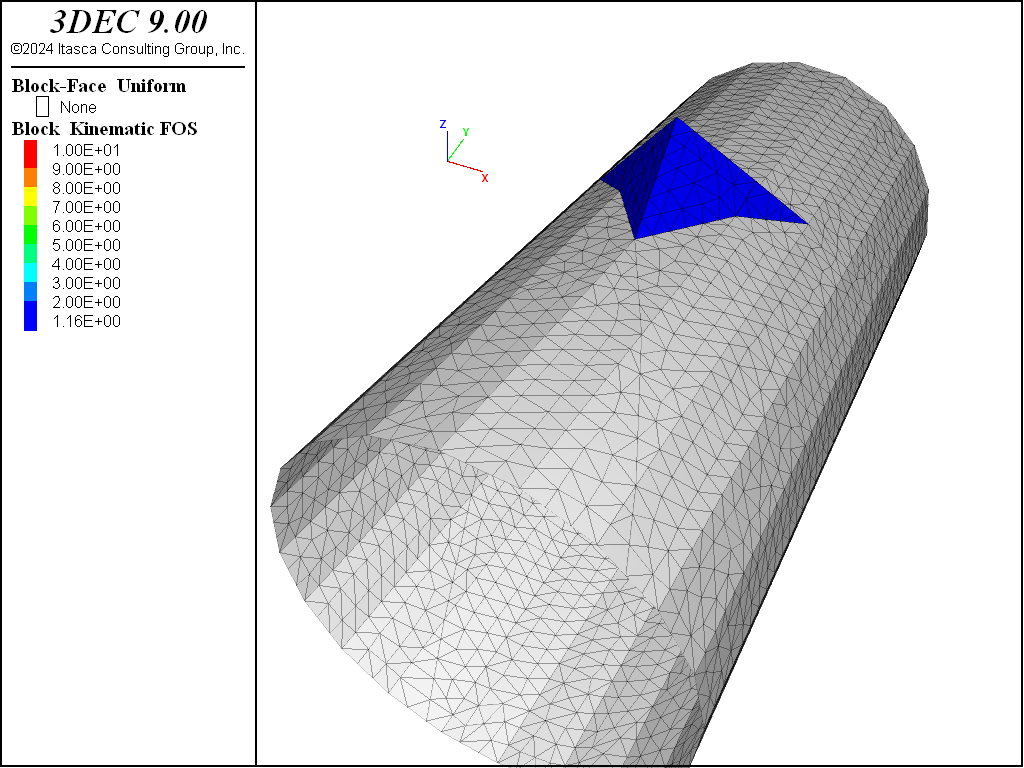
Figure 4: Kinematic factor of safety distribution on wedge block faces for the case \(K_0=1\) and \(k_n/k_s=10\).

A1.dat

model new

; Geometry
block create brick -10. 10. -10 10 -10 10

fish define table_definition 

  ; Define a cylinder with radius = 5m. A point is defined every 18 degrees

  local theta=0.
  local i=1
  local rad=5.
  local delta_theta=18

  loop while theta<360.
    local x1=rad*math.cos(theta*math.degrad)
    local y1=rad*math.sin(theta*math.degrad)
    table.value('1',i)=vector(x1,y1)
    i=i+1
    theta=theta+delta_theta
  endloop 
end
[table_definition]

block group "rock_mass"
block cut tunnel table-1 '1' table-2 '1' axis 0,-10,0 0,10,0 ...
                                         radial group "tunnel"

; Cut a tetrahedral block 
block cut joint-set dip 60. dip-direction 0. origin 0. 0. 7.
block cut joint-set dip 60. dip-direction 120. origin 0. 0. 7.
block cut joint-set dip 60. dip-direction 240. origin 0. 0. 7.

block zone generate edgelength 0.5

; Install stress in MPa
block zone cmodel assign elastic
block zone property density 2500e-6
model gravity 9.81

block insitu topography ratio-x 1 ratio-y 1 overburden [-190*9.81*2500e-6]

; now mark faces and delete tunnel
block face group "free" range group-intersection "rock_mass" "tunnel"
block delete range group "tunnel"

; now work out FOS forigin given joint properties (MPa)
block analyze-stability free-face 'free' ...
  stiffness-normal 10000 stiffness-shear 1000 cohesion 0 friction 35
  
block group 'wedge' range plane  dip 60 dip-direction 0 origin 0 0 7 below ...
                        plane  dip 60 dip-direction 120 origin 0 0 7 below ...
                        plane  dip 60 dip-direction 240 origin 0 0 7 below ...
                        position-z 3.5 10

Parametric Study on Block Stability and Comparison to 3DEC Rigid Blocks

A parametric study is performed using the isolated block stability method on the block from the preceding example. The ratio \(K_0\) is varied for different values of \(k_n/k_s\). When using the isoblock method, a FISH function is used to vary the stresses and run the tests because the same model can be used over and over.

The results are analyzed in terms of safety factor for the wedge block (the mean FOS computed on block faces). The mean of the face FOS values for a block can be stored in the block’s extra variable by using the keyword block-extra with the block analyze-stability. In this example, the FOS is stored in block extra variable 1.

Figure 5 shows the results. For \(k_n/k_s\) = 1, the block is stable for all tested values of \(k_0\). For \(k_n/k_s\) = 10, the block will fall for \(k_0\) < 0.8. For \(k_n/k_s\) = 100, the block will fall for \(k_0\) < 1.

The advantage of using the block stability-analyze command over a typical 3DEC model is that the result is obtained instantaneously (no need to “solve”). Also, the typical 3DEC model would need to be much larger to set the boundaries far from the region of interest.

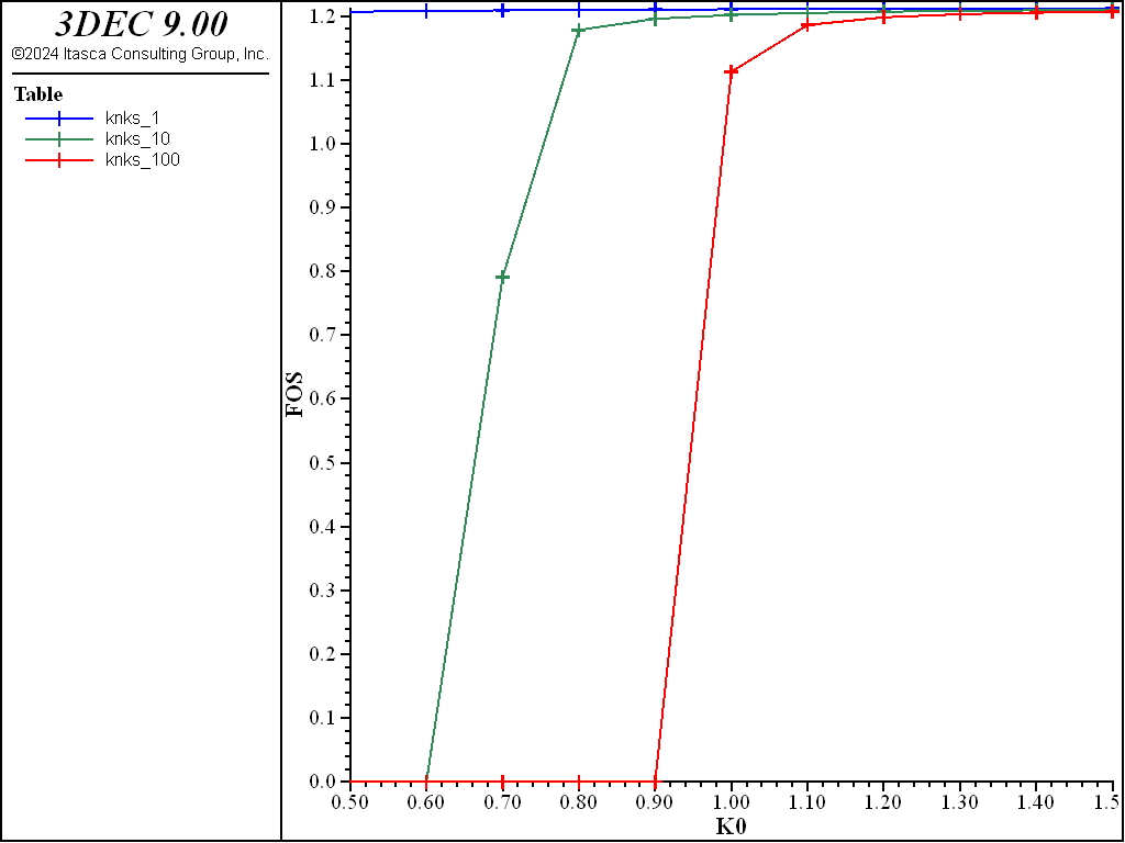
Figure 5: Results of the mean safety factor per block using isolated block stability. Note that FOS = 0 represents a block failing by tension.

02_A2run.dat

model restore 'A2_geometry'

; now test different stress ratios and joint stiffnesses
fish define test

  ks = 1000 ; shear stiffness
  phi = 35 ; friction angle
  count = 0
  
  ; try three different kn/ks ratios
  loop i (1,3)
    factor = 10.0^(i-1)
    kn = ks * factor   ; 1, 10 , 100
    tablename = 'knks_'+string(factor)
    tab_ = table.create(tablename)
    
    ; now test different initial stresses
    K0_list = list.seq(0.5,0.6,0.7,0.8,0.9,1,1.1,1.2,1.3,1.4,1.5)
    
    szz = -5.0 ; MPa
    szz_grad = 2500e-6*9.81  ; density 2500, gravity 9.81
    
    loop foreach K0 K0_list
      ; install stresses and run FOS test
      command
        block zone initialize stress-xx [szz*K0] gradient 0 0 [szz_grad*K0] 
        block zone initialize stress-yy [szz*K0] gradient 0 0 [szz_grad*K0]
        block zone initialize stress-zz [szz] gradient 0 0 [szz_grad]
        block analyze-stability free-face 'free'  stiffness-normal [kn] ...
          stiffness-shear [ks] friction [phi] block-extra 1
      end_command
      
      ; get min block FOS (assume it is the wedge)
      minfos = 1e12
      loop foreach block block.list
        if block.group(block,'isolated_block') # "None"
          minfos = math.min(minfos,block.extra(block,1))
        endif
      endloop
      
      ; add to table
      count = count + 1
      table.value(tab_,count) = vector(K0,minfos)
      
    end_loop
  end_loop
end

[test]

table 'knks_1' export 'knks_1.tab'
table 'knks_10' export 'knks_10.tab'
table 'knks_100' export 'knks_100.tab'

Tunnel with Multiple Blocks

This example considers block stability for several blocks located around a tunnel. The blocks are generated by introducing a DFN (Figure 6) with the following properties: uniform orientation, uniform size (set to 50 m), density of 2.

The tunnel size, joint properties, and tunnel depth are the same as in the previous examples. Given that only blocks touching the tunnel will be studied using the isolated block stability method, the model extents are limited to a cube of 20 m width.

After running the command block analyze-stability, blocks touching the tunnel are assigned a group name in slot “isolated_blocks.” The group name is equal to the block ID (or leader ID if joined). So the blocks touching the tunnel can be plotted by hiding the blocks if the “isolated_block” group equals “none” (Figure 7).

The mean FOS for every block is printed on the graphical interface, and can be stored by specifying a block-extra as described previously in the second example. Figure 8 shows unstable blocks (having a mean FOS < 1).

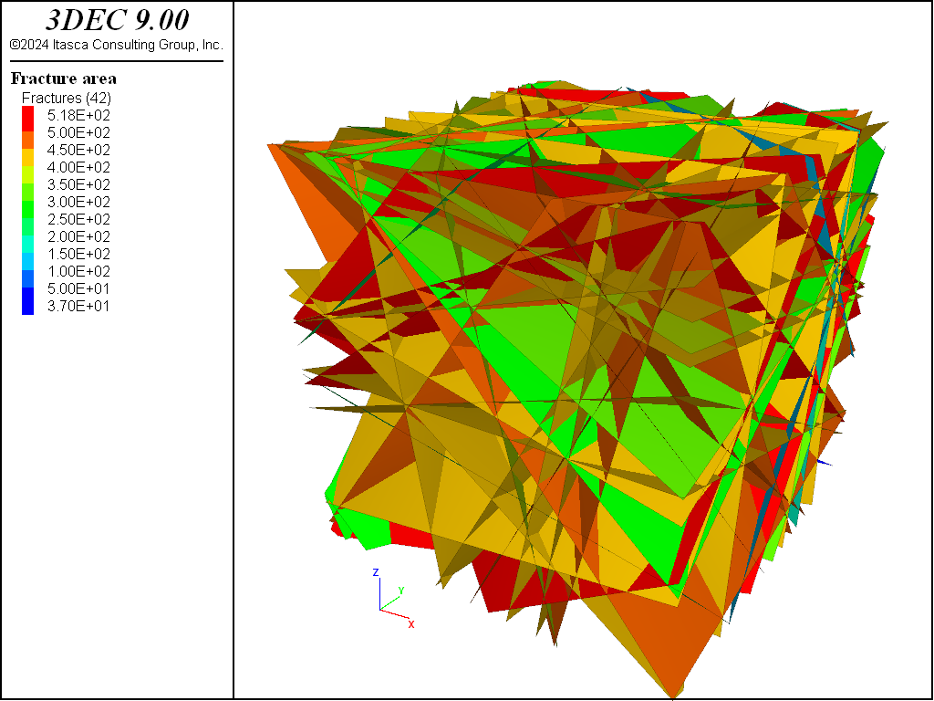
Figure 6: Discrete fracture netowrk used to create the block model.

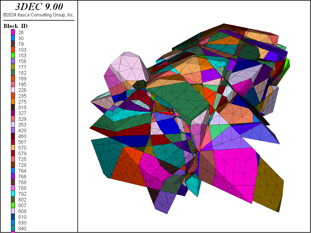
Figure 7: Identified free blocks (stored in group slot “isolated_block”).

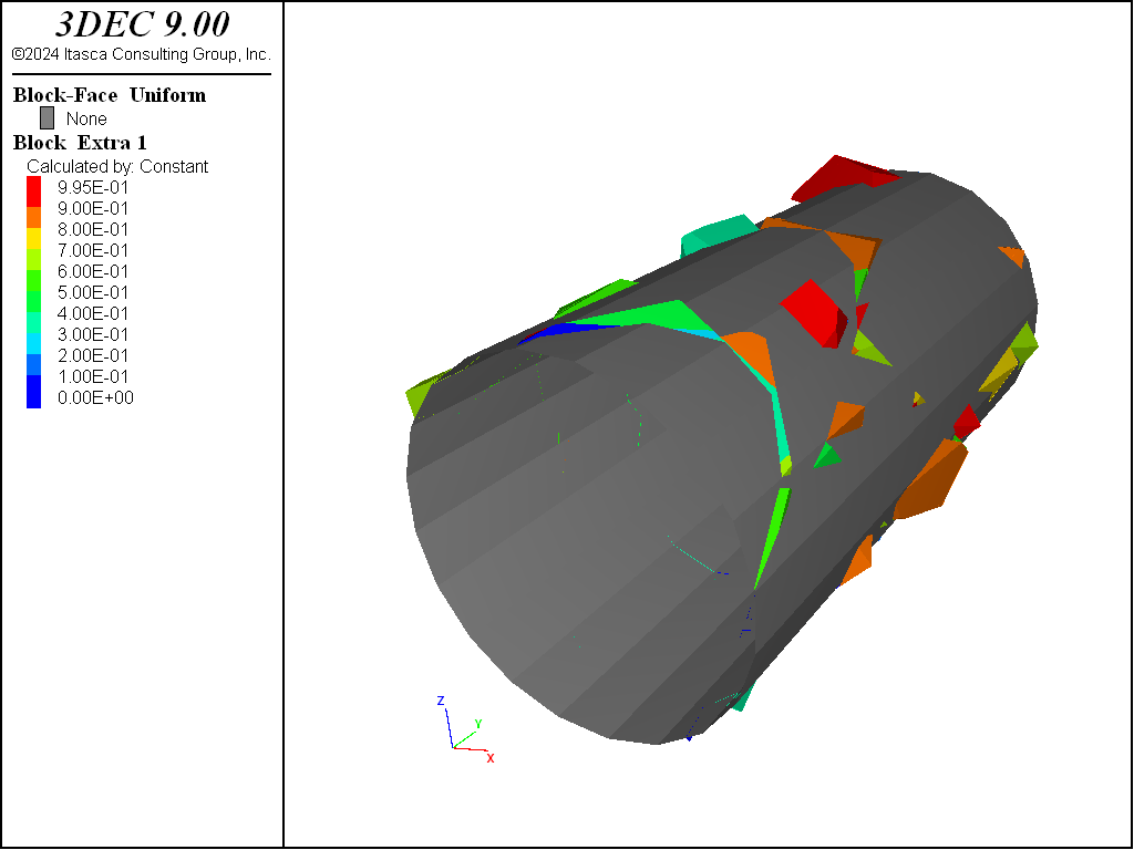
Figure 8: Unstable blocks (with FOS_mean ≤ 1).

A3.dat

model new

; Geometry
block tolerance 1e-3
block create brick -10. 10. -10 10 -10 10

model domain extent -10. 10.

model random 10000

; Define DFN template 
fracture template create 'fractures' orientation uniform ...
     size uniform size-limits 50 50
     
fracture generate dfn 'fractures' template 'fractures' mass-density 2


fish define table_definition 

  ; Define a cylinder with radius = 5m. A point is defined every 18 degrees

  local theta=0.
  local i=1
  local rad=5.
  local delta_theta=18

  loop while theta<360.
    local x1=rad*math.cos(theta*math.degrad)
    local y1=rad*math.sin(theta*math.degrad)
    table.value('1',i)=vector(x1,y1)
    i=i+1
    theta=theta+delta_theta
  endloop 
end
[table_definition]

block group "rock_mass"
block cut tunnel table-1 '1' table-2 '1' axis 0. -10. 0. 0. 10. 0. ...
                                         radial group "tunnel"

; Cut joints
block cut dfn name 'fractures'

block zone generate edgelength 1.0 

; Install stress in MPa.  Use K0 = 0.5
block zone cmodel assign elastic
block zone property density 2500e-6
model gravity 9.81

block insitu topography ratio-x 0.5 ratio-y 0.5 overburden [-190*9.81*2500e-6]

; now delete tunnel
block face group "free" range group-intersection "rock_mass" "tunnel"
block delete range group "tunnel"

model save 'A3_mesh'

block analyze-stability free-face 'free' stiffness-normal 10000 ...
                                         stiffness-shear 1000   ...
                                         friction 35 block-extra 1

block hide on range group  'isolated_block=none' 

model save 'A3_K0_0.5'

References

Ghazal, R., F. Hadj-Hassen, and M. Tijani. (2011) “A new numerical method to study isolated blocks around underground excavations taking into account in-situ stresses,” in Proceedings, 45th US Rock Mechanics / Geomechanics Symposium (San Francisco, California, June 2011). Alexandria, Virginia: ARMA.

Ghazal, R. (2013) Modélisation de la stabilité des blocs rocheux sur la paroi des excavations souterraines avec prise en compte des contraintes initiales et du comportement non linéaire des joints. PhD thesis. Ecole des Mines de Paris.

Ghazal, R., F. Hadj-Hassen, and M. Tijani. (2011) “Stability modelling of isolated rock blocks at the surface of underground excavations taking into account in-situ stresses”. In Proceedings, 12th ISRM Congress (October 2011, Beijing, China), Harmonising Rock Engineering and the Environment Zhou Y, editor.

Goodman, R. E., G. H. Shi. (1985) Block theory and its application to rock engineering. NJ:Prentice-Hall, editor. Englewood Cliffs.

Warburton, PM. (1985) A computer program for reconstructing blocky rock geometry and analyzing single block stability. Computers & Geosciences 11(6), 707 – 712.