Joint Fluid Flow

Introduction

Rock joints have been extensively studied, both experimentally and analytically, because of their influence on the overall mechanical and hydraulic behavior of rock masses. The joint is an interface between two rock surfaces, and the hydromechanical behavior of the joint is controlled primarily by the roughness of the two surfaces. Roughness is a function of the genesis of the joint. Tensile fractures, for example, have a more pronounced roughness than fractures that have experienced some shear deformation. The narrow zone of rock in the immediate vicinity of a joint (including the joint itself) exhibits significantly different hydromechanical behavior than the “intact” rock away from the joint. Thus:

The deformability of the joint (per unit “thickness” of the joint) is much larger than the deformability of the intact rock. The roughness of the two surfaces in contact makes the area of actual contact much smaller than the area of overlap between the two surfaces involved in the contact.
The shear strength of the rock mass in the plane of the joint is much smaller than the shear strength of the intact rock. The joints are discontinuities in the material and the resistance to shear deformation is due predominantly to friction and the roughness of the surfaces in contact.
The cross-sectional area of a joint is much larger than the cross-sectional area of pores within the intact rock. Consequently, fluid flow rates through joints are several orders of magnitude larger than flow rates through the pores in the intact rock. However, the porosity of unfractured blocks is distributed throughout the rock mass, so that the matrix porosity is much larger than the rock mass porosity due to the joints. Thus, fluid flow in the rock mass is controlled by the joints, while most of the fluid is stored in the pores within the intact rock.

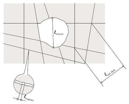
../../../../../_images/jointflow-length.png — Figure 1: Length scales in models of a rock mass.

The length scale of joint roughness is much smaller than the length scales of both the joint and of an engineering structure (see the figure above):

(1)\[\begin{split}\begin{align} l_{roughness} & << l_{rock\ block} \\ \\ l_{roughness} & << l_{structure} \end{align}\end{split}\]

When analyzing practical problems under conditions such as defined by the relations in Equation (1), a model that explicitly represents the geometry of the joint roughness on the scale of an engineering structure would be extremely inefficient: details of the joint roughness should be ignored whenever possible. In a model on the scale of a rock block and/or an engineering structure, joints should be analyzed as two-dimensional[1] (or one-dimensional if the model is two-dimensional) discontinuities characterized by constitutive relations and related properties on the macro scale (e.g., normal and shear stiffness, friction, dilation, hydraulic aperture). The joint macro properties are related to a “point” of a joint which, in fact, represents an area of the joint, termed the “Representative Elementary Area” or REA, with a characteristic length that is much larger than the characteristic length of the joint surface roughness \(l_{roughness}\), and much smaller than the characteristic length of the model (\(l_{rock\ block}\) or \(l_{structure}\)). The macro properties and variables defined on the level of REA (i.e., the result of the integration of micro effects) represent inhomogeneity of the joint parameters as a smoothly varying function of the position \(x_{i}\) in the joint plane (see Figure 2).

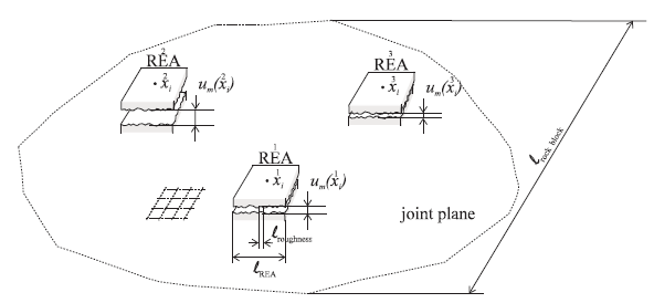
../../../../../_images/jointflow-rea.png — Figure 2: REA and inhomogeneity in the joint plane.

Joint Hydraulics and Parallel Plate Model for Incompressible Flow

The governing equations for fluid flow in joints follows a simplified form of the Navier-Stokes equation. When the Navier-Stokes equation for fluid flow between two almost parallel, impermeable boundaries is combined with the condition of incompressibility of the fluid, it simplifies to the Reynolds equation (Batchelor 1967):

(2)\[\Bigl({{u^3 \rho g} \over {12 \mu}} \phi, _i \Bigr), _i = 0\]

where: \(u = (x_i)\) is the distance between the impermeable boundaries at some point \(x_i\) (\(i = 1,2\)) in the plane; \(\phi = z + p/\rho g\) is the hydraulic head; \(g\) is the acceleration due to gravity; \(\rho\) is the fluid density; \(\mu\) is the fluid viscosity; \(z\) is the elevation; and \(p\) is the pressure in the fluid. Equation (2) is integrated over the distance between the impermeable boundaries. For joint surfaces between rock blocks, Equation (2) is integrated over the thickness of the thin, planar interface, separating two blocks.

For Equation (2) to be valid, the flow must be laminar (i.e., fluid should flow in parallel layers). The Reynolds number is a dimensionless number that describes whether flow conditions lead to laminar or turbulent flow,

(3)\[Re = {{\rho u_c v_{\rm max}} \over {\mu}}\]

where \(u_c\) is the characteristic cross-sectional dimension and \(v_{\rm max}\) is the maximum velocity of the fluid. The Reynold’s number gives a measure of the ratio of inertial forces to viscous forces, and consequently quantifies the relative importance of these two types of forces for given flow conditions.

Equation (2) is valid, as long as inequality Equation (4) is satisfied.

(4)\[\alpha {{\rho u_c v_{max}} \over {\mu}} << 1\]

where \(\alpha\) is the angle between the two surfaces enclosing the fluid. In essence, the condition expressed by Equation (4) ensures that the flow remains laminar. From Equation (2), the fluid flow rate per unit width of the plates may be written as

(5)\[q_i = - {{u^3 \rho g} \over {12 \mu}} \phi, _i = - k_H \phi, _i\]

where the permeability of a single fracture is \(u^2/12\), and the hydraulic conductivity is \(k_H = \rho gu^2/12 \mu\).

Note that application of Equation (5) is suitable for cases where flow is occurring dominantly in fractures, or planar flow channels of very small thickness. If flow is occurring through large void spaces of irregular three-dimensional shape between the solid blocks, this approach is no longer suitable.

Range of Validity of Parallel Plate Model, Hydraulic Aperture, and Mechanical Aperture

In Equation (2), \(u(x_i)\) is the actual distance between two rough surfaces of the joint at the point xi . Typically, in the boundary value problems, variation of the joint aperture occurs on a much smaller scale than the characteristic length of the model (e.g., the block size, or characteristic length of the engineering structure), and it is useful to obtain a relation between \(q_i\) and \(\phi, _i\) that is valid on the macro scale of the joint, but which neglects (when possible) the local variations of aperture. A first guess is to develop a relation of the same form as that of Equation (2), except that uh is now a macro parameter related to the REA of the joint surface — i.e.,

(6)\[q_i = {{u^3_h \rho g} \over {12 \mu}} \phi, _i\]

where \(u_h(x_i)\) is the hydraulic aperture of the joint related to the REA. However, the validity of Equation (6) as a model of fluid flow through a rock joint has been questioned by many researchers. There is general agreement that (6) can be valid over a certain range of \(u_h\) only. Thus:

Upper bound: When \(u_{h}\) increases such that the Reynolds number becomes larger than a critical value, flow becomes turbulent. Iwai (1976) determined that the critical Reynolds number for a rock joint is \(Re\) = 100, while Louis (1974) determined the critical number to be \(Re\) = 2300.
Lower bound: The hydraulic aperture \(u_{h}\) of the joint cannot be reduced mechanically to zero (i.e., there is some residual flow through a joint even under very high stresses). During the closure of mismatched joints, the area of actual contact between the two surfaces increases, but never becomes equal to the nominal area of the joint. The mismatched roughness forms channels in the joint plane under high compressive stresses: flow becomes localized and very much dependent on the details of the joint roughness, which is abstracted on the macro level of the REA. Realistically, under such conditions, it is not even possible to define the REA. This poses serious problems for modeling: the response of the model is controlled by geometrical details which have a characteristic length that is much smaller than the characteristic length of the model (see Figure 1).

The major reason for the argument against the validity of the fluid flow model expressed by Equation (6) (within the previously mentioned lower and upper limits) is the difficulty in determining the hydraulic aperture, \(u_h\). The hydraulic aperture, \(u_h\), is a function of the mechanical aperture, \(u_m\), which is defined as the average distance between the joint surfaces. It is difficult to measure the mechanical aperture directly. Most authors assume that \(u_h = u_m\). (A summary of the published results of joint conductivity testing has been given by Alvarez et al. (1995).) The initial aperture, \(u_{m0}\), is the aperture at the beginning of the loading cycle. Some authors equate this initial aperture with the maximum joint displacement during the compression, while others measure the residual flow rate at maximum joint closure, and, from this, calculate the residual aperture (from (6)), adding it to the maximum closure to calculate the initial mechanical and hydraulic aperture. Comparison of the measured flow rates in a joint with those predicted by the model (given by Equation (6)) using the calculated hydraulic aperture (as a function of the mechanical aperture) very often show significant disagreement. Witherspoon (1980) proposed the following form of the “cubic law”:

(7)\[q_i = - {{u^3_m \rho g} \over {12 \mu F}} \phi, _i\]

where \(F\) is a correction factor. Comparing Equation (6) and Equation (7), we obtain:

\[u_h = f u_m\]

\[f = {1 \over {F^{1/3}}}\]

Detournay (1980) has proposed a relation between the hydraulic aperture, \(u_h\), and the joint deformation, \(\Delta u_m\):

(8)\[u_h = f u_m = u_{h0} + f \Delta u_m\]

This permits a more general fitting of the “cubic law” to experimental results. The joint conductivity, \(k_H\), is defined (assuming one-dimensional flow):

(9)\[k_H = - {q \over {d \phi/dx}}\]

Assuming the following dependence of the joint conductivity on hydraulic aperture:

(10)\[k_H = {{\rho g} \over {12 \mu}} (u_{h0} + f \Delta u_m)^3\]

we obtain

(11)\[u_{h0} + f \Delta u_m = - \Bigl({{12 \mu} \over {\rho g}} {{q} \over {d \phi/dx}} \Bigr)^{1/3}\]

The unknown parameters \(u_h0\) and \(f\) can be calculated by linear regression of the experimental results. The validity of the model given by Equation (7) and Equation (11) for a particular data set can also be verified by linear regression. Alvarez et al. (1995) have reanalyzed some previously published data on joint conductivity, and have confirmed the validity of the “modified cubic law” as given by Equation (11).

The flow rate is a function of the joint closure for two reasons:

the area (in cross-section) through which the fluid flows is reduced as the joint closes; and
the area of actual contact between two joint surfaces increases, making the flow more tortuous.

The parameter \(f\) reflects the influence of the roughness on the tortuosity of the flow. For smooth or interlocking joints, \(f\) is approximately 1.0; for mismatched joints with a small ratio of span to roughness height, \(f\) has values smaller than 1.0.

Hydromechanically Coupled Fluid-Flow Formulation in Rock Masses

The problem of fluid flow in rock masses is a hydromechanically coupled problem. That is, fluid pressures affect the mechanical deformation, and mechanical deformation affects pressures. There are three aspects of hydromechanical coupling in a fractured rock mass:

the effect of pore pressure on deformation and strength of fractured rock masses;

the effect of mechanical deformation on permeability; and

the effect of mechanical deformation on pore pressures.

In a hydromechanically coupled formulation in a discrete fracture network, the effect of mechanical deformation on permeability arises as a result of the change in opening of the fractures.

Effect of Pore Pressure on Deformation and Strength

The fluid pressure in the fracture affects the fracture normal deformation. When the rock fracture is filled with fluid under a certain pressure (Figure 3), the normal deformation of the fracture is a function of a linear combination of the confining pressure (or total normal stress) in the rock, \(\sigma_n\), and the fluid pressure, \(p_p\). Any linear combination of \(\sigma_n\) and \(p_p\) that produces the same fracture deformation is termed an “effective stress,” \(\sigma'_n\), of the fracture. Walsh (1981) derived an expression for the effective stress from the condition that there is no change of pore space volume as a function of the normal stress and the pore pressure:

(12)\[dv_p = -{{\delta v_p} \over {\delta p}} (d \sigma_n + d p_p) + v_p \beta_s dp_p = 0\]

where \(v_p\) is the volume of pore space, and \(\beta_s\) is the compressibility of the rock around the fracture. The first term in Equation (12) is the deformation of the dry fracture due to a “confining” stress equal to \(d \sigma_n + d p_p\) (the compressive stress is negative; the fluid pressure is positive), while the second term is equal to the increase of pore space in the fracture due to a hydrostatic pressure equal to \(d p_p\) (Figure 3). The expression for effective stress can be obtained (Walsh 1981) from Equation (12), as

(13)\[d \sigma'_n = d \sigma_n + (1 - {{v_p \beta_s} \over {\delta v_p / \delta p}}) d p_p\]

or, in simplified form,

(14)\[\sigma'_n = \sigma_n + \alpha p_p\]

The effective stress coefficient \(\alpha\) has been measured in experiments to be in the range of 0.5 < \(\alpha\) < 1.0. Smaller values of \(\alpha \sim\) 0.5 are measured for tensile fractures with rough surfaces, while larger values (i.e., \(\alpha \sim\) 1.0) are measured when the fracture surfaces are smooth.

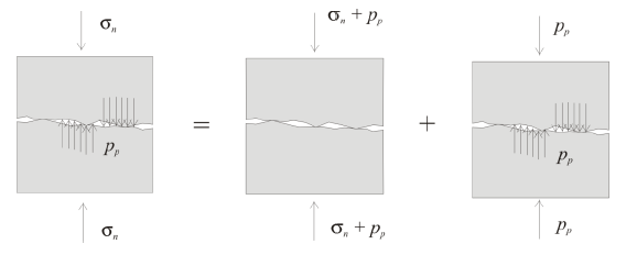
../../../../../_images/jointflow-fracturedef.png — Figure 3: Normal fracture deformation.

The pore pressure also affects the strength of the rock fractures through the effective stress principle. Both tensile and shear failure conditions of the rock fractures are expressed in terms of the effective, not total, stress. However, when the effective stress is used for assessment of normal or shear strength of rock fractures, it always is defined as \(\sigma'_n = \sigma_n + p\) (i.e., the effective stress coefficient is always equal to 1).

Effect of Mechanical Deformation on Permeability

The mechanical aperture, \(u_m\), which is defined as the average distance between the fracture surfaces, is a function of mechanical deformation. Clearly, the hydraulic aperture, \(u_h\), used in calculation of flow rate in the rock fractures in Equation (6), is a function of the mechanical aperture \(u_m\). However, comparison of the measured flow rates in a fracture with those predicted by the model (given by Equation (6)) using the hydraulic aperture assumed to be equal to the mechanical aperture very often show significant disagreement. The relations of hydraulic aperture and mechanical aperture, and their effects on permeability change are discussed in Range of Validity of Parallel Plate Model, Hydraulic Aperture, and Mechanical Aperture.

Effect of Deformation on Pore Pressures

The continuity equation for a slightly compressible fluid in a deformable rock fracture has the form:

(15)\[q_{i,i} = - {{\delta u} \over {\delta t}} - {{u} \over {K_w}} {{\delta p} \over {\delta t}}\]

Combining Equation (5) and Equation (15), assuming \(u = u_m = u_h\) and that \(u\) does not vary as a function of position, we obtain the expression

(16)\[{{\delta p } \over {\delta t}} = {{u^2 K_w} \over {12 \mu}} p_{i,i} - {K_w \over u} {{\delta u} \over {\delta t}}\]

which is the diffusion equation for the pressure inside the fracture. In the general case, the fracture aperture, \(u\), is not only the function of the local fracture stiffness and fluid pressure, but also of the mechanical response of larger volume of the rock mass. Therefore, the term \((K_w / u)(\delta u / \delta t)\) in Equation (14) is external, or a “source,” which is determined by coupling between fluid flow and mechanical deformation of the solid model. This term represents the pressure change in the water “trapped” (i.e., under undrained conditions) within the rock fracture due to deformation of the rock mass and rock fractures in particular.

3DEC Joint Model

Constitutive Model and Relevant Properties

As discussed in the previous sections, the models that characterize the constitutive response of joints can be complicated. The model implemented in 3DEC, however, uses a simple approximation of joint behavior.

In 3DEC, normal and shear joint stiffness are represented by linearly elastic springs. The shear resistance of the joint is usually characterized by the Coulomb slip law. Dilational response can be represented by prescribing a dilation angle.

For fluid flow simulation within joints, three additional parameters representing the constitutive response of joint apertures with respect to effective stress must be defined by users. The aperture-effective stress constitutive response implemented in 3DEC is relatively simple, and is schematically shown in Figure 4. The relation between hydraulic aperture and effective stress is basically a bilinear curve with the effective stress coefficient \(\alpha\) (defined in Equation (14)) assumed to be 1.0.

The hydraulic aperture is given, in general, by

(17)\[u_h = u_{h0} + \Delta u_n\]

where \(u_{h0}\) is the joint aperture at zero normal stress; and \(\Delta u_n\) is the joint normal displacement (positive denoting opening). Joint aperture is also bound by a lower value, \(u_{res}\), which is the minimum (residual) value for the aperture, below which mechanical closure does not affect the contact permeability. For this model, the aperture at zero stress, \(u_{h0}\), and the residual hydraulic aperture, \(u_{res}\), must be defined by the users. Note that \(u_{h0}\) can also be the joint aperture at the in-situ stress state if the nodisplacements keyword is used with the block insitu command, or if the residual aperture, \(u_{res}\), is set equal to \(u_{h0}\) when in-situ streses are applied.

In addition to zero and residual values of hydraulic aperture, a maximum value, \(u_{max}\), may also be assumed, for efficiency, in the explicit calculation. The maximum value sets the maximum value that is used in flow rate calculation. However, mechanical apertures are always calculated by adding the differential normal displacement to the zero value aperture (i.e., \(u_m = u_{h0} + \Delta u_n\) and can be larger than \(u_{max}\)). In defining the dependence of the joint conductivity on hydraulic aperture (see Equation (10)), it is assumed that \(f\) = 1.0. This means that the mechanical aperture is equal to the hydraulic aperture except when the mechanical aperture exceeds \(u_{max}\).

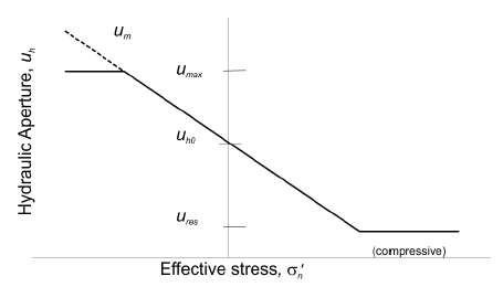
../../../../../_images/jointflow-appvstress.png — Figure 4: Idealized relation between hydraulic aperture and effective normal stress for a rock joint. Effective stress is positive in compression on this plot.

During solution, at each timestep of the 3DEC mechanical calculation, the computations determine the updated geometry of the system, thus yielding the new values of apertures for all contacts (refer to “Mechanical Calculations for Motion and Interaction in 3D”). Flow rates through the contacts are calculated from Equation (6) considering the upper bound for aperture, \(u_{max}\).

Pressures are calculated and stored in a data structure called a flow knot (see Geometrical and Topological Model of a Fractured Rock Mass). Subsequent to flow rate calculations, the flow-knot pressures are updated, taking into account the net flow into the flow knot and possible changes in flow-knot volume due to the incremental motion of the surrounding blocks. The new flow-knot pressure becomes

(18)\[p = p_0 + K_w Q {{\Delta t} \over {V}} - K_w {{\Delta V} \over {V_m}}\]

where:

\(p_0\) is the flow-knot pressure in the preceding timestep;

\(Q\) is the sum of flow rates into the flow-knot from all surrounding contacts;

\(K_w\) is the bulk modulus of the fluid;

\(\Delta V = V - V_0\); and

\(V_m = (V + V_0) / 2\), where \(V\) and \(V_0\) are the new and old flow-know volumes, respectively.

If the new domain pressure computed by Equation (18) is negative, then the pressure is set to zero (i.e., negative pressures cannot exist).

Degree of Saturation

In the current version of 3DEC, joints are assumed to be fully saturated and the degree of saturation is always one (1). Pore pressures can be positive or zero (0). No negative pore pressures are possible.

Fluid Timestep Size and Numerical Stability

In explicit time integration techniques, the timestep size cannot exceed the critical timestep. Numerical stability of the present explicit fluid flow algorithm requires that the fluid timestep, \(\Delta t_f\), be limited to

(19)\[\Delta t_f = {\rm min} [{{V} \over {K_w \Sigma_i k_i}}]\]

where \(V\) is flow-knot volume, and the summation of permeability factors, \(k_i\), is extended to all contacts surrounding the flow-knot.

The minimum value of \(\Delta t_f\) over all flow knots is the critical timestep in the analysis. For transient flow analysis, the numerical stability requirements may be rather severe, and may make some analyses very time-consuming or impractical, especially if large contact apertures and very small flow-knot volumes are present. Furthermore, the fluid inside a joint also increases the apparent joint stiffness by \(K_w / u_h\), thus possibly requiring a reduction of the timestep used in the mechanical calculation. In an explicit algorithm, this implies that the mechanical timestep must be reduced.

The fluid timestep, calculated by Equation (19) is inversely proportional to the fluid bulk modulus and joint transmissivity, which is proportional to aperture cubed. For typical joint apertures, fluid timesteps on the order of milliseconds are obtained. Therefore this algorithm can only be applied in practical problem settings to short duration simulations. See Tips for Speeding Up Coupled Simulations for discussion on increasing the timestep for practical analyses.

Calculation Modes and Commands for Fluid-Flow Analysis

Fluid-Only Analysis

It is possible to model the fluid flow in the joints without considering the effect of the fluid pressures on rock deformation, or the effect of rock mass deformation on diffusivity of the fluid. This form of analysis will be called “uncoupled” or “fluid-only,” because specific storage is controlled by fluid compressibility only and rock mass is assumed to be infinitely stiff.

A fluid flow analysis may be transient (in which time is important), or steady-state (in which only the pressures at very long times are required). In 3DEC, the solution is always transient. If a steady state solution is desired, the transient problem is simply run until pore pressures are no longer changing, at which time steady-state is assumed to have been achieved. Note that reducing the fluid bulk modulus in a flow-only analysis will not speed up the calculation. Reducing the modulus will increase the timestep, but will also increase the time required to reach steady-state. Therefore, for a steady-state analysis, the choice of \(K_w\) is unimportant.

For a transient analysis, the choice of \(K_w\) is important to get the correct time scale. If correct bulk modulus of fluid is used, that means that rock mass is rigid and its deformability on time scale of the diffusion process is completely neglected. However, under certain conditions it is possible to conduct flow-only simulation but account for deformability of the rock mass (i.e., storage related to rock deformation) by reducing the used fluid bulk modulus. In such a way, it is possible to have correct time scale in the model without running sometimes time-consuming coupled simulations. The rate of pressure propagation in a saturated medium is dictated by the diffusivity:

(20)\[c = {{k_H} \over S}\]

where \(k_H\) is the hydraulic conductivity (units of length/time), \(S\) is the storage (units of 1/length). If the stiffness of the joint is neglected, the storage in a jointed, saturated material can be given by

(21)\[S = \rho_w g \Bigl({{u_h / s} \over {K_w}} + {{1} \over {K + 4/3 G}}\Bigr)\]

where \(u_h\) is the hydraulic aperture, \(s\) is the joint spacing, \(K_w\) is the true fluid bulk modulus, and \(K\) and \(G\) are the rock bulk and shear moduli, respectively. Because it is assumed that the rock is rigid in a fluid-only analysis, the second term in Equation (21) is zero. To account for the rock deformation, we can use an apparent fluid bulk modulus as shown:

(22)\[K^{a_w} = {{u_h / s} \over {{u_h / s} \over {K_w}} + {{1} \over {K + 4/3 G}}}\]

Using this value in a fluid-only analysis will give the correct storage Equation (21) and therefore the correct diffusivity Equation (20) and time scale.

To solve a fluid flow problem in 3DEC, first the fluid flow analysis must be turned on in the beginning of the model set-up so that additional data structures for fluid flow memory requirements are created (i.e, the configuration command for fluid flow (model config fluid) should precede all other commands). For a fluid-only analysis, the fluid analysis must be activated and the mechanical analysis must be deactivated (model fluid active on and model mechanical active off). The required fluid material properties for fluid are density, viscosity and bulk modulus. For joint material properties, only the initial aperture (\(u_{h0}\)) is required since there is no mechanical calculation and the apertures will not change. However, the user must still specify the residual aperture and maximum aperture since otherwise they will default to zero. These can be set the same as \(u_{h0}\). An example model of flow only through a single joint is shown in Example flow_only.3ddat. The apparent fluid modulus is calculated from Equation (22), assuming a true fluid bulk modulus of 2 GPa and a joint spacing of 2 m.

The fluid pressure and discharge on the joint are shown in Figure 5. To create this plot, add the plot items Flow Planes / Contours / Pore Pressure / and Fluid Vectors / Discharge, then rotate to see the joint plane. Figure 6 shows the evolution of pressure in the middle of the joint. You can see that steady state is reached after about 12 s of time.

flow_only.3ddat

model new
model configure fluid
model large-strain off

block create brick -1 1 -1 1 -1 1
block cut joint-set dip 0 dip-direction 90

block zone generate edgelength 0.25
block zone cmodel assign elastic
block zone property density 2500 shear 2e9 bulk 5e9 

block contact jmodel assign mohr
block contact property stiffness-normal 1e10 stiffness-shear 1e10

block fluid property bulk 3.8e5
block fluid property density 1000
block fluid property viscosity 1e-3

flowplane vertex property aperture-initial 1e-4 aperture-minimum 1e-4 ...
                          aperture-maximum 1e-4 

flowknot apply pore-pressure 5.0e6 range position-x -1
flowknot apply pore-pressure 0 range position-x 1
;
model history fluid time-total
flowknot history pore-pressure position 0 0 0
;
model fluid active on
model mechanical active off
model cycle 1000
;

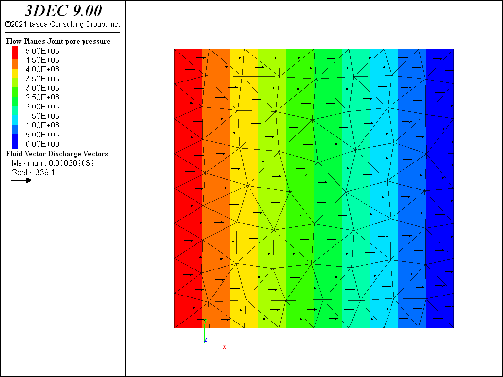
../../../../../_images/flowonly_pressure.png — Figure 5: Fluid pressures and discharge vectors on the joint.

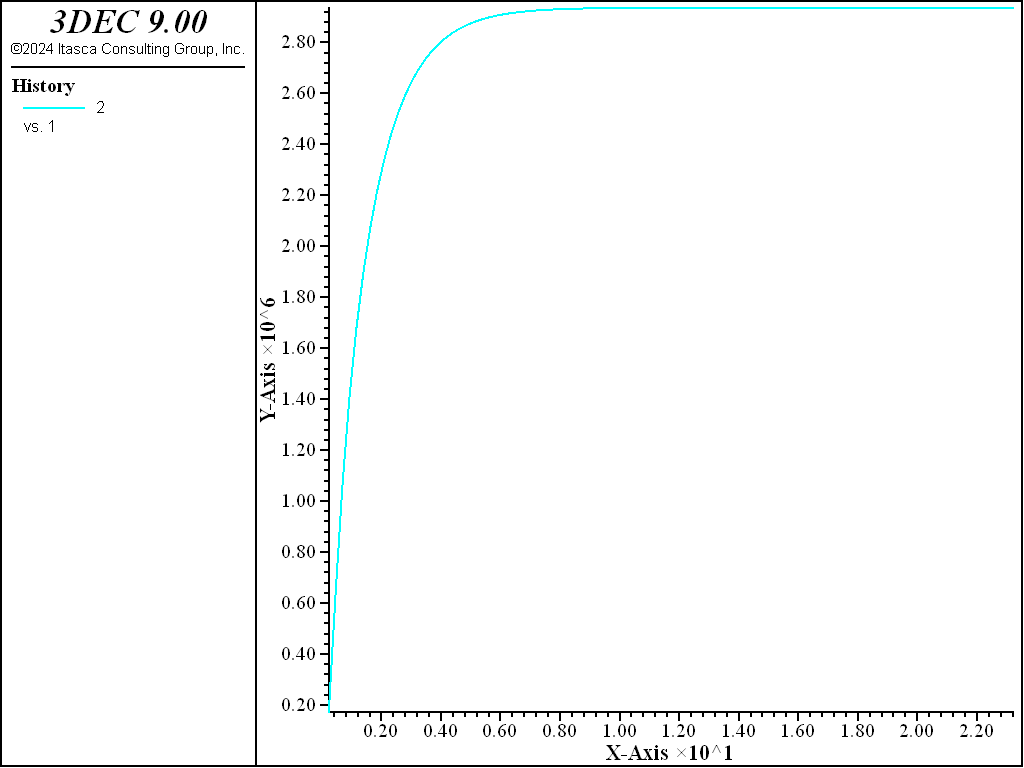
../../../../../_images/flowonly_history.png — Figure 6: History of pressure in the middle of the joint.

One-Way Coupling

If pressure changes and the mechanical deformation are weakly coupled (i.e., the pressure changes do not cause significant aperture changes), and particularly when we are not interested in the transient response of the model, the problem can be simulated as a one-way coupled, by sequential execution of flow only and mechanical only simulations.

Once a flow-only analysis has been completed (Fluid-Only Analysis), a mechanical analysis can be done in which the fluid pressure changes will influence the mechanical behavior. Changing fluid pressures will change the effective stress on the joints, and this will cause the (elastic and/or inelastic) deformation of the solid model. The effective stress is used in calculation of joint failure condition, so changes in normal effective stress (due to changes in fluid pressure) will move the stress state in the joint relative to the failure surface as shown in Figure 7.

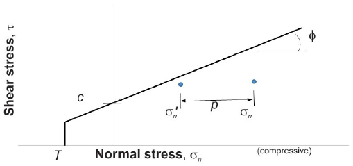
../../../../../_images/coupled_relation.png — Figure 7: Effect of fluid pressure on sliding condition for the failure envelope for a joint with cohesion, \(c\), and friction angle \(\varphi\).

The one-way coupling analysis requires the same properties as the fluid-only analysis (fluid bulk modulus, viscosity and density). As with the fluid flow only analysis, the residual and maximum apertures are unimportant and can be set to the same as \(u_{h0}\).

The one-way coupled analysis requires the following steps:

Specify an in-situ stress state and pore pressure. Solve for an initial mechanical stress state. To do this, it is necessary to set \(K_w\) = 0, so that fluid pressures do not change due to rock deformation. The mechanical-only calculation is performed using model fluid active off and model mechanical active on.
Set up fluid boundary conditions using flowknot apply pore-pressure, flowknot apply discharge, flowplane edge apply discharge. By default, boundaries are impermeable.
Solve for the fluid pressures as in Fluid-Only Analysis. Use model fluid active on and model mechanical active off and set the fluid bulk modulus to \(K_w^a\) from Equation (22).
Solve for the effect of the fluid pressures on the solid by again using model fluid active off and model mechanical active on, and setting \(K_w\) = 0.

An example is shown below. Note that in this example, the pore pressure is not initialized. The pore pressures are generally initialized, usually based on the location of a water table. The example creates a model with a single joint and sets up an initial isotropic stress in the blocks of 10 MPa. A fluid pressure of 11 MPa is then applied to the left side, and pressure is held at zero on the right side. The displacement contours induced by the pressure changes are shown in Figure 8.

one_way.dat

model new
; one-way coupled simulation
model configure fluid
model large-strain off

block create brick -1 1 -1 1 -1 1
block cut joint-set dip 0 dip-direction 90

block zone generate edgelength 0.25
block zone cmodel assign elastic
block zone property density 2500 shear 2e9 bulk 5e9 

block contact jmodel assign mohr
block contact property stiffness-normal 1e10 stiffness-shear 1e10 

block fluid property bulk 3.8e5
block fluid property density 1000
block fluid property viscosity 1e-3

flowplane vertex property aperture-initial 1e-4 ...
                          aperture-minimum 1e-4 aperture-maximum 1e-4 

;
block gridpoint apply velocity-x 0 range position-x -1
block gridpoint apply velocity-x 0 range position-x 1
block gridpoint apply velocity-y 0 range position-y -1
block gridpoint apply velocity-y 0 range position-y 1
block gridpoint apply velocity-z 0 range position-z -1
block gridpoint apply velocity-z 0 range position-z 1
;
block insitu stress -1e7 -1e7 -1e7 0 0 0

model fluid active off
model mechanical active on
block fluid property bulk 0.0

model history mechanical unbalanced-maximum

model cycle 100

model fluid active on
model mechanical active off
;
flowknot apply pore-pressure 1.1e7 range position-x -1
flowknot apply pore-pressure 0.0 range position-x 1
;
block fluid property bulk 3.8e5

history delete
model history fluid time-total
flowknot history pore-pressure position 0 0 0

model cycle 1000
model fluid active off
model mechanical active on
block fluid property bulk 0.0
model cycle 1000
program return

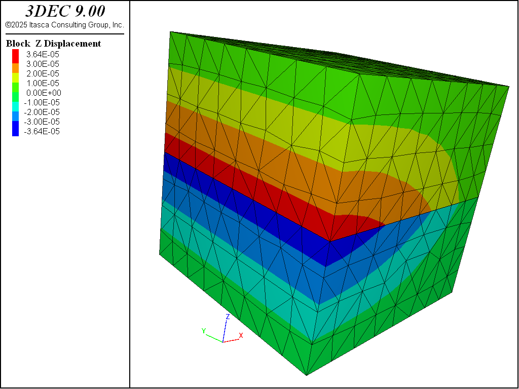
../../../../../_images/coupled_zdisp.png — Figure 8: \(z\)-displacements in the block after one-way coupled analysis.

Undrained

The preceding example is one-way coupled because the fluid pressures affect the deformation but the solid displacements do not affect the fluid pressure (after the initial stress installation). Another example of simplified coupling is when deformation is not induced by diffusion-related pore-pressure changes but by mechanical loading occurring on relatively short time-scale such that pore-pressure diffusion can be neglected. This is generally called an undrained deformation.

The undrained analysis requires the following steps:

Set up initial stresses and pore pressures as in the one-way coupled case.
Specify realistic values for \(u_{res}\) because the joint aperture affects the deformation-induced pore pressure changes.
Set the fluid bulk modulus to the true bulk modulus of fluid (e.g., 2 GPa). Use model fluid active off and model mechanical active on to perform mechanical calculations. The pore pressures will change as the joint aperture changes as shown by the third term in Equation (18).

An example is shown below. In this example, the initial stress and pore pressure are initialized to zero. Stress is then applied on the top of the sample, and the pore pressures on the joint increase accordingly. The joint is then sheared to show how the pore pressures on the joint affect the shear strength.

The induced fluid pressures on the joint are shown in Figure 9. The pressures are generally close to 1 MPa, indicating that the applied mechanical stress is taken up by the fluid. The \(x\)-displacements in the blocks during the shear are shown in Figure 10. The shear stresses in the joint plane during shear are negligible because the effective normal stress on the fault is close to zero, facilitating slipping of the fault.

undrained.dat

; undrained deformation
model new
model configure fluid
model large-strain off
;
block create brick -1 1 -1 1 -1 1
block cut joint-set dip 0 dip-direction 90

block zone generate edgelength 0.25
block zone cmodel assign elastic
block zone property density 2500 shear 2e9 bulk 5e9

block contact jmodel assign mohr
block contact property stiffness-normal 2e9 stiffness-shear 2e9 ...
                       friction 30. tension 1e30

block fluid property bulk 2.e9
block fluid property density 1000
block fluid property viscosity 1e-3

flowplane vertex property aperture-initial 1e-4 ...
                          aperture-minimum 1e-15 aperture-maximum 1
;
block gridpoint apply velocity-x 0.0 range position-x -1
block gridpoint apply velocity-x 0.0 range position-x 1
block gridpoint apply velocity-y 0.0 range position-y -1
block gridpoint apply velocity-y 0.0 range position-y 1
block gridpoint apply velocity-z 0.0 range position-z -1
;
; Assume in-situ stress is 0.  Apply stress to top.
block face apply stress 0 0 -1e6 0 0 0 range position-z 1
;
model fluid active off
model mechanical active on

; local damping is better forigin undrained analysis
block mechanical damping local

model solve
model save 'undrained-load'
;
; Apply shear
block gridpoint apply-remove velocity-x range position-x -1.1 1.1
block gridpoint apply velocity-x 0.01 velocity-z 0.0 range position-z 0.1 1.1
block gridpoint apply velocity-x 0.0 range position-z -1
block contact history stress-shear position 0 0 0
block gridpoint initialize displacement 0 0 0
model cycle 2500
program return

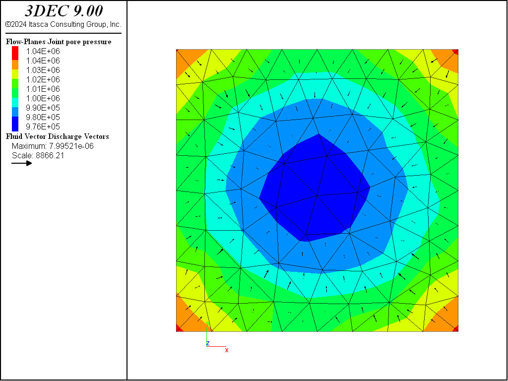
../../../../../_images/undrained_pressure.png — Figure 9: Pore pressures on the joint after loading under the undrained conditions.

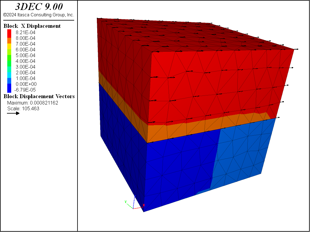
../../../../../_images/undrained_xdisp.png — Figure 10: \(x\)-displacements in the blocks.

Fully Coupled Hydromechanical Simulation

In many cases, (e.g., fluid pressure changes cause solid deformation sufficient to result in aperture changes large compared to the initial apertures), fully coupled hydromechanical simulation is required. In this scenario, the solid deformations influence the fluid pressures, and the fluid pressures also affect the mechanical stresses and strains. The solution is performed by alternating frequently between mechanical and fluid calculations. The user has control over the number of mechanical steps executed per fluid step (or vice versa) as described below.

The subsections below outline the steps required when performing a fully coupled analysis.

Definition of Fluid Properties

The fluid material properties required for analysis are density, viscosity and bulk modulus (commands block fluid property density, block fluid property viscosity, and block fluid property bulk). For joint hydraulic properties, aperture-initial, aperture-minimum, and aperture-maximum representing aperture at zero stress, residual aperture and maximum hydraulic aperture must be specified. This is done with the flowplane property command.

Solving for Initial State

First specify an in-situ stress and pore pressure (using command block insitu). For solving for the initial state, first the mechanical mode is activated and the flow is turned off (model fluid active off and model mechanical active on) and the fluid bulk modulus is set to 0 (block fluid property bulk 0). These steps ensure that the stress solution is obtained without changing the fluid pressures. After equilibrium is obtained, the mechanical mode is turned off, flow is turned on (model fluid active on and model mechanical active off) and fluid bulk modulus is set back to its true value. The problem is then stepped to equilibrium again to obtain the initial steady-state pressures. During initialization, the goal is to initialize equilibrium stresses and steady-state pressures within the model. The displacements that occur during this step are typically meaningless (i.e., not a consequence of a physical process) and therefore once the initial state is obtained, the displacements should be reset (block gridpoint initialize displacement 0 0 0 and block contact reset displacement).

The keyword nodisplacement may be used during the stress installation with the block insitu command. nodisplacement prevents normal displacements (due to initial stress) from being subtracted from aperture-initial (zero stress hydraulic aperture). Consequently, azero will be the initial and not the zero-stress apertures.

Running the Coupled Solution

To run a coupled solution, both mechanical and flow mode must be on. Internally, 3DEC runs a series of mechanical steps followed by a series of fluid steps. The number of mechanical step per each fluid step and the number of fluid step per each mechanical step can be set by the users.

In most cases, the time associated with mechanical deformation is significantly less than that associated with fluid flow. In fact, the assumption of the coupled hydromechanical model in 3DEC is that it is quasi-static. The mechanical model is in equilibrium for the current distribution of pore pressures. Consequently, although both flow and mechanical model are explicitly integrated in time, only flow time is physical time. Furthermore, the flow and mechanical models do not need to be synchronized. For each flow timestep, it is sufficient conduct as many mechanical timesteps as needed to achieve the mechanical equilibrium. Equilibrium is assumed to have been reached when the maximum unbalanced force falls below a given threshold. By default, the threshold is 1 × 10⁻⁵. This can be changed with the mechanical ratio maximum keyword in the model solve command.

Sometimes reaching the unbalanced force threshold for each flow timestep can be very time-consuming. Therefore, it is also possible to specify the maximum number of mechanical cycles to be executed per fluid timestep. By using the command model mechanical follower on and command model mechanical substep 200, the maximum number of mechanical cycles to be executed between fluid flowsteps is set at 200 irrespective of the unbalanced force. The actual number of executed mechanical steps may be less if the mechanical model comes to equilibrium in less than 200 steps. This command simply prevents the execution of an excessive number of mechanical steps per fluid step.

In some cases, particularly for long times after the initial perturbation to the model, the pressure changes and perturbations to the mechanical within one flow timestep can be relatively small. In those circumstances, executing one or more mechanical steps per one flow timestep could be unnecessary and inefficient. In this case, the command model fluid follower on and command model fluid substep n can be used to set the maximum number of fluid timesteps executed per mechanical step to n (the default is 1).

Example

The following example is similar to the one-way coupled example, except that now fully coupled hydromechanical simulation is performed.

After running this example, it can be seen that over 500,000 steps have been executed. This is because multiple mechanical steps are performed for each fluid step (20,000 fluid steps are executed as specified in the file). The total time is only about 0.047 s. Figure 11 shows the pressure contours in the joint. It is clear that the steady-state solution has not been reached (compare to Figure 5) and that pressures are still changing. The joint aperture contours are shown in Figure 12. This plot is generated by adding the plot item Flow PLane / Contours / Aperture. Finally, the block displacement contours are shown in Figure 13. This plot indicates that the blocks are deforming in response to the fluid pressure changes, and that the model is indeed coupled.

coupled.dat

; fully coupled analysis
model new
model configure fluid
model large-strain off

block create brick -1 1 -1 1 -1 1
block cut joint-set dip 0 dip-direction 90

block zone generate edgelength 0.25
block zone cmodel assign elastic
block zone property density 2500 shear 2e9 bulk 5e9

block contact jmodel assign mohr
block contact property stiffness-normal 1e10 stiffness-shear 1e10 

block fluid property bulk 2e9 density 1000 viscosity 1e-3

flowplane vertex property aperture-initial 1e-4 ...
                          aperture-minimum 1e-5 aperture-maximum 1e-3

block gridpoint apply velocity-x 0.0 range position-x -1.0
block gridpoint apply velocity-x 0.0 range position-x  1.0
block gridpoint apply velocity-y 0.0 range position-y -1.0
block gridpoint apply velocity-y 0.0 range position-y  1.0
block gridpoint apply velocity-z 0.0 range position-z -1.0
block gridpoint apply velocity-z 0.0 range position-z  1.0

block insitu stress -1e7 -1e7 -1e7 0 0 0 nodisplacements
block insitu pore-pressure 2e6

; initial equilibrium - mechanical
model fluid active off
block fluid property bulk 0.0
model history mechanical unbalanced-maximum
model cycle 100

; inital equilibrium - fluid
model fluid active on
model mechanical active off
block fluid property bulk 2e9
model cycle 100

block gridpoint initialize displacement 0 0 0
block contact reset displacement

flowknot apply pore-pressure 3.0e6 range position-x -1.0
flowknot apply pore-pressure 2.0e6 range position-x 1.0

model mechanical active on
block fluid property bulk 2e8

model mechanical substep 10
model mechanical follower on

history delete
model history fluid time-total
flowknot history pore-pressure position 0 0 0

model solve fluid cycles 20000 or mechanical ratio 1e-5

model save "coupled"

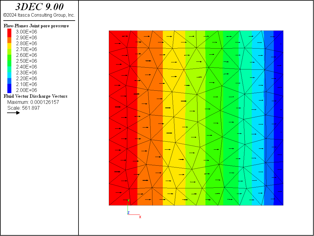
../../../../../_images/coupled_pressure.png — Figure 11: Fluid pressures in the coupled model after 20,000 steps.

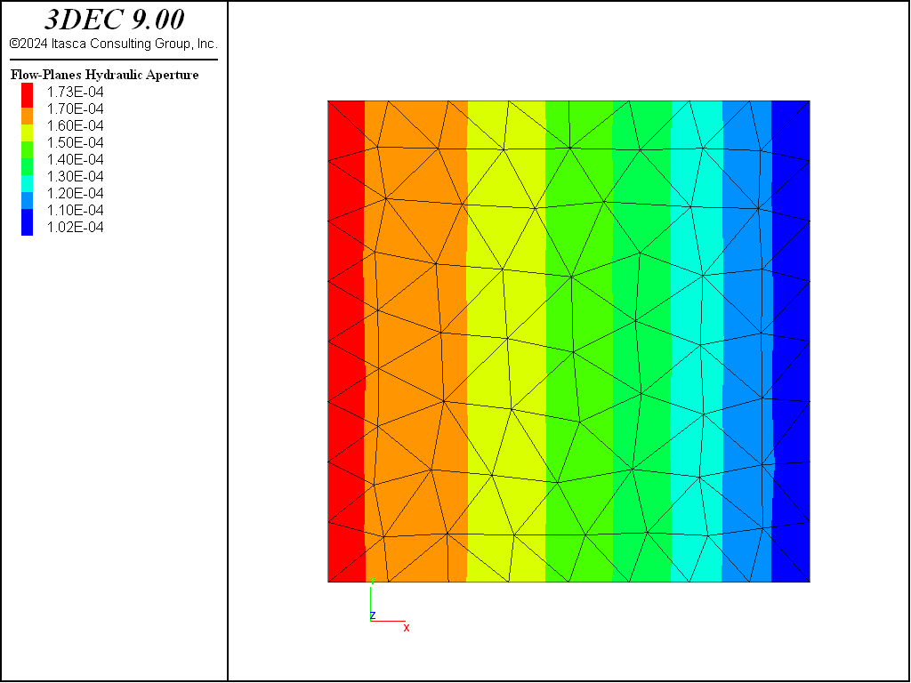
../../../../../_images/coupled_aperture.png — Figure 12: Joint apertures in the coupled model after 20,000 steps.

Fast Flow

A fast-flow option is provided to speed up the coupled calculations. This option assumes that the fluid is incompressible. This may be a reasonable assumption when the rock is not very stiff relative to the fluid, or if the apertures are very small. Recall that the apparent joint stiffness (if saturated) is \(K_w / u_H\). Therefore, a small aperture will yield a large apparent stiffness, such that it may be possible to assume that the stiffness is essentially infinite (i.e., fluid inside the joint is incompressible).

The fast-flow option is activated with the command block fluid fast-flow active on. Note that in general, the fast-flow logic will produce much larger fluid timesteps, so a larger value for model mechanical substep may need to be used to ensure mechanical equilibrium is reached (approximately) each step.

The fast-flow logic also requires a different value for fluid bulk modulus. The fluid is assumed to be incompressible, so instead of a true modulus for the fluid, a quantity must be provided as input that is equal to the material bulk modulus divided by the cube of the zone size (i.e., K/edge³). When fastflow is on, this quantity (that has SI dimension of Pa/L³) is input using the command block fluid bulk property \< value \> . For models with variable material properties and zone sizes, the maximum value for this parameter should be used.

The example “coupled.dat” is modified in “coupled-fast.dat” to use the fast-flow logic. The following changes are required:

The fluid bulk modulus is set to the solid bulk modulus divided by the cube of the zone size.
The number of possible mechanical steps per fluid step is increased to 2000.
The fluid time step is limited to a maximum of 1e-3 s.

If the fluid timestep is not limited, then the initial fluid timestep is quite large. This results in a large initial pressure pulse and unstable behavior in the model. With the timestep limited to 1e-3 s, the timestep is still approximately 1000 times larger than in the example with no fast flow. Therefore, only about 200 fluid steps are required to reach the steady state (approximately 50,000 total steps). This is significantly less than the non-fast-flow version shown above.

coupled-fast.dat

; fully coupled analysis with fast-flow
; fully coupled analysis
model new
model configure fluid
model large-strain off

block create brick -1 1 -1 1 -1 1
block cut joint-set dip 0 dip-direction 90


block zone generate edgelength 0.25
block zone cmodel assign elastic
block zone property density 2500 shear 2e9 bulk 5e9

block contact jmodel assign mohr
block contact property stiffness-normal 1e10 stiffness-shear 1e10 

flowplane vertex property aperture-initial 1e-4 ...
                          aperture-minimum 1e-5 aperture-maximum 1e-3

block fluid property bulk 2e9 density 1000 viscosity 1e-3

block gridpoint apply velocity-x 0.0 range position-x -1.0
block gridpoint apply velocity-x 0.0 range position-x  1.0
block gridpoint apply velocity-y 0.0 range position-y -1.0
block gridpoint apply velocity-y 0.0 range position-y  1.0
block gridpoint apply velocity-z 0.0 range position-z -1.0
block gridpoint apply velocity-z 0.0 range position-z  1.0

block insitu stress -1e7 -1e7 -1e7 0 0 0 nodisplacements
block insitu pore-pressure 2e6

; initial equilibrium - mechanical
model fluid active off
block fluid property bulk 0.0
model history mechanical unbalanced-maximum
model cycle 100

; inital equilibrium - fluid
model fluid active on
model mechanical active off
block fluid property bulk 2e9
model cycle 100

block gridpoint initialize displacement 0 0 0
block contact reset displacement 

flowknot apply pore-pressure 3.0e6 range position-x -1.0
flowknot apply pore-pressure 2.0e6 range position-x 1.0

block fluid fast-flow active on

model mechanical active on
block fluid property bulk [2e9/0.25^3]
model mechanical substep 2000 
model mechanical follower on

history delete
model history fluid time-total
flowknot history pore-pressure position 0 0 0

model fluid timestep maximum 1e-3
model solve fluid cycles 250 or mechanical ratio 1e-6

model save "coupled-fast"

Leak-off

With matrix fluid flow on, it is possible to simulate the migration of fluid from the joints to the adjacent rock blocks (leak-off). By specifying model configure matrixflow, both the joint fluid flow and the matrix flow will be on. Flow knots will be created at each gridpoint location in the matrix. At flow plane locations, one flow-knot represents two (or more) coincident gridpoints, so that the joint flow and matrix flow are connected.

An example is shown below. This is a fluid-only calculation – there is no fluid-mechanical coupling. Therefore the bulk modulus of the fluid in the matrix is set to the apparent fluid bulk modulus calculated by equation (22). If the matrix fluid bulk modulus is not given with the block fluid property bulk-matrix command, then the matrix fluid bulk modulus is set the same as the joint fluid bulk modulus (given with the block fluid property bulk command).

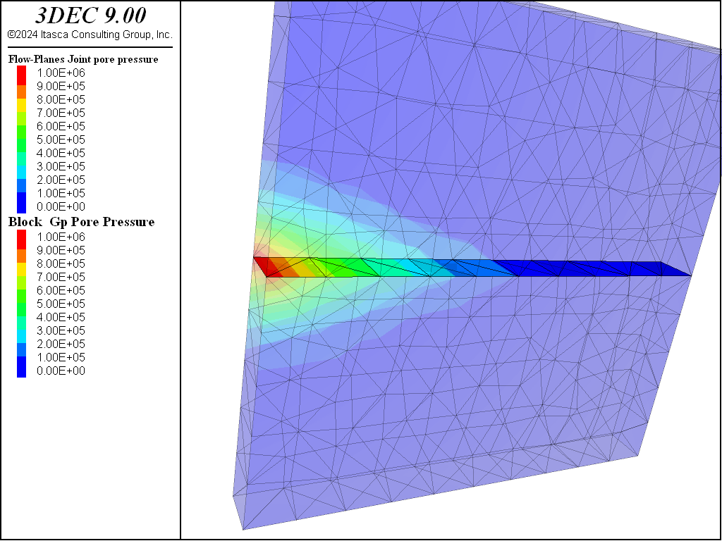
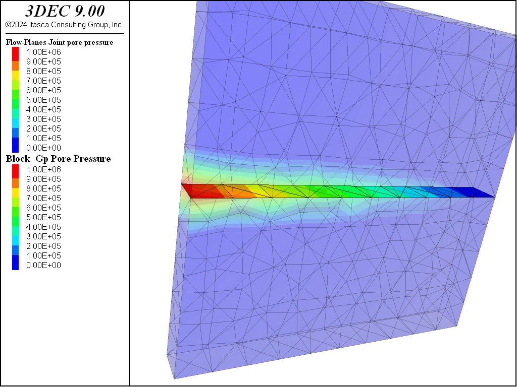
For the first example, the matrix permeability is set to 1×10⁻⁶ m/s. The pore pressures after 1.5 s are shown in Figure 14. It is clear that fluid has migrated from the fracture into the matrix. Figure 15 shows the same example with matrix permeability set to 1 × 10⁻⁸ m/s. In this case, the fluid does not migrate as far into the matrix and consequently flows farther along the joint.

../../../../../_images/leakoff-pressure-1.png

../../../../../_images/leakoff-pressure-2.png

leakoff-1.dat

program log on
program log-file 'leakoff-1.log'
; --------------------------------------------------------
; leakoff-1   ... matrix conductivity 1e-6 m/s
; --------------------------------------------------------
;
model new
model configure matrixflow
model large-strain off
;
block create brick -5 5 -0.5 0.5 -5 5
block cut joint-set
;
block zone generate edgelength 1.0
block zone cmodel assign elastic
block zone property density 2500 shear 1e9 bulk 2.5e9 

block contact jmodel assign mohr
block contact property stiffness-normal 1e11 stiffness-shear 1e11 
flowplane vertex property aperture-initial 2e-4 ...
                          aperture-minimum 2e-4 aperture-maximum 2e-4 

block fluid property bulk 2e9 density 1000 viscosity 1e-3

; perm = (1e-6 m/s) / (rho*g) = 1e-10
block zone fluid property permeability 1e-10
block zone fluid property porosity 0.10
;
block insitu stress 0 0 -1e6 0 0 0
;
block gridpoint apply velocity-x 0 velocity-y 0 velocity-z 0 ...
                      range position-z -5
;
flowknot history pore-pressure position -5 0 0
flowknot history pore-pressure position -2 0 0
flowknot history pore-pressure position 0 0 0
flowknot history pore-pressure position 2 0 0
flowknot history pore-pressure position -2 0 5
flowknot history pore-pressure position 0 0 5
flowknot history pore-pressure position 2 0 5
flowknot history pore-pressure position -2 0 -5
flowknot history pore-pressure position 0 0 -5
flowknot history pore-pressure position 2 0 5
flowknot history pore-pressure position -5 -1 0
flowknot history pore-pressure position -5 1 0
flowknot history pore-pressure position -3 -1 0
flowknot history pore-pressure position -3 1 0
flowknot history pore-pressure position -5 -1 1
flowknot history pore-pressure position -5 1 1
flowknot history pore-pressure position -5 -1 -1
flowknot history pore-pressure position -5 1 -1
;
; forigin fluid only analysis, compute apparent fluid bulk modulus
fish define kf_matrix
  local poros_ = 0.1
  local rockbulk_ = 2.5e9
  local shear_ = 1e9
  local fluidbulk_ = 2e9
  
  kf_matrix = poros_/(poros_/fluidbulk_ + 1.0/(rockbulk_+4.0/3.0*shear_))
end
block fluid property bulk-matrix [kf_matrix]
;
flowknot apply pore-pressure 1e6 range position-x -5 position-z 0
flowknot apply pore-pressure 0.0 range position-x 5 position-z 0
;
model fluid active on
model mechanical active off
model solve fluid time-total 1.5
;
flowknot list range position-z -0.1 0.1
;
model save 'leakoff-1'

Considerations for Model Optimization

Based on the discussion presented in the preceding section, the characteristics of a coupled hydromechanical model lead to the following two distinct difficulties that modelers confront:

The fluid trapped in a joint appears to be very stiff, due to the small aperture. In other words, the apparent stiffness of the filled joint is determined by the term \(K_w / u_h\), which is often very large because of relatively small apertures. The large apparent fluid stiffness results in small mechanical and flow timesteps.
Permeability is a very sensitive function of joint aperture, owing to the cubic term in the flow equation. Consequently, aperture increase results in sharp reduction in the fluid timestep.

These two difficulties are addressed separately.

The problem with large fluid bulk modulus is that typically the diffusivity of the problem is controlled by the deformability of the rock mass (i.e., fluid bulk modulus does not affect the physics of the problem). On the other hand, the fluid bulk modulus is used in the calculation of the timesteps, resulting in very small timesteps. To mitigate this problem, it is suggested that the fluid bulk modulus be reduced. For example, water bulk modulus at 20° is approximately 2.2 GPa. Considering typical joint apertures, the apparent stiffness of the water-filled joints is many orders of magnitude higher than the rock stiffness. If such contrast in stiffness exists in the model, it is suggested that the fluid bulk modulus be reduced such that the apparent stiffness of fluid-filled joint is approximately equal to the equivalent stiffness of the adjacent zone in the block representing the rock.

Localized large displacement can drastically reduce the fluid timestep. Capping the aperture aperture-maximum in the flow rate calculations can prevent the effect of such large apertures on the timestep without affecting the physics of the analyzed problem. However, it is suggested that the maximum aperture is chosen such that it does not affect the aperture in a relatively large part of the flow model.

Tips for Speeding Up Coupled Simulations

Aside from using fast-flow, other possible approaches for speeding up the coupled calculations include:

Setting a lower value for model mechanical substep or a higher value for mechanical ratio. Either of these changes may reduce the number of mechanical steps per fluid step. Again, care should be taken not to reduce the number of mechanical steps too much or the blocks will not properly deform in response to fluid pressure changes.
Use the command flowplane area-minimum to set the minimum permissible flow plane area. It is possible during discretization that very small zones within the flow planes may form, with an area much smaller than the average zone area. These zones will drastically reduce the flow timestep. If there is relatively small number of such small zones, it is possible to assign them area-minimum (i.e., treat them in the calculations as if their area is area-minimum), resulting in significant increase in the timestep, with relatively small effect on the physics of the simulated problem. However, if area-minimum affects a relatively large number of zones in the model, this parameter is not correctly selected because it will be affecting the physics of the simulated problem. To determine the value to use for area-minimum, a FISH function could be written to generate a histogram of flow plane areas, and then a suitable value that truncates the smallest values (e.g., two standard deviations below the mean) could be chosen.
Use the command flowknot volume-minimum to set the minimum knot volume. Knot volumes, which are much smaller than the mean knot volume, can be created during block geometry generation and/or during discretization and significantly affect the fluid timestep. If there is a relatively small number of such knots with small volumes, it is possible to assign them volume-minimum (i.e., treat them in the calculations as if their volume is volume-minimum) resulting in significant increase in the timestep, with relatively small effect on the physics of the simulated problem. However, if volume-minimum affects relatively large number of knots in the model, this parameter is not correctly selected because it will be affecting the physics of the simulated problem. To determine the value to use for volume-minimum, a FISH function could be written to generate a histogram of flow knot volumes, and then a suitable value could be chosen that truncates the smallest values (e.g., two standard deviations below the mean).
Use the command flowplane zone edge-minimum to set the minimum flow zone edge length. All zones with edges below this value are “deactivated” (with a flag). They are not deleted, and the user can change the minimum value later (or set it to zero to revert to the standard logic). By deactivating very small edges, the timestep will increase as discussed above.
Use block fluid fast-flow active on. See above for details.
Reduce aperture-maximum. See advice above.
Reduce the fluid bulk modulus. Note that reducing the fluid modulus will cause the fluid to be more deformable, so the fluid will have a smaller effect on the mechanical behavior than would be true in reality, and the volume balance (inflow versus fluid content) will not be exactly correct. The fluid bulk modulus can be intelligently reduced on flowknots that are causing small timesteps by using the block fluid timestep command. Please see this command for details, including the warnings.

Representation of a Discrete Fracture Network (DFN) for Fluid Flow Simulations

Discrete fractures in a rock mass generally are the result of loadings that have occurred at different times in the geological history of the rock mass. The fractures, usually planar and extensive, can be identified as belonging to specific sets — each with characteristic orientation and spacing. It is impossible to know the geometry of the whole fracture network. Therefore, many fracture models are stochastic. Relevant statistical properties of a network are computed from observable quantities, and then are used to generate stochastic fracture fields. Such models are strictly three-dimensional, because connectivity properties simply cannot be scaled between two and three dimensions. (For further information on discrete fracture networks, please refer to DFN overview.)

Although the limitation of 3DEC block geometry requires that blocks cannot be partially fractured, such an effect (of partially fractured blocks) can be achieved by assigning variable properties to the sub-contacts within the contact surfaces between two blocks. Consequently, part of the joint plane could be assigned higher strength and behave as the “rock bridge,” or intact rock material, and part could be assigned strength of frictional surfaces and behave as the rock joint, or surface of weakness. The fractures may be represented as circular discs or as polygons.

For each fracture, a joint plane will cut though all blocks intersected by the fracture. Because partially fractured blocks cannot exist in 3DEC, the joint plane associated with a fracture extends to the boundaries of associated blocks (see Figure 16).

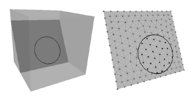
../../../../../_images/leakoff-subcontacts.png — Figure 16: Illustration of how sub-contacts on a joint plane can be assigned different properties inside (black) and outside (gray) of a circular fracture.

After cutting, 3DEC does not differentiate between the fracture and the joint plane. To define a fracture with a particular shape, a second step is required. Once block generation is complete, and the model is discretized into tetrahedral zones, the fractured and unfractured part of the joint plane is differentiated by assigning different material properties (see Section 6.6 in the User’s Guide). CS: see previous flag – same idea

Under default conditions, flow can occur within all joint planes. However, because in reality flow can only occur through the fractures, then it is necessary to prevent flow from occurring in the unfractured parts of the joint plane. This can be achieved by turning on the option of crackflow in 3DEC using the command block fluid crack-flow on. By turning this option on, flow can occur only through the yielded (either in shear or tension) part of the joint planes. In order to allow flow to occur in the DFN when crackflow is turned on, the sub-contacts within the fracture need to be assigned a failure indicator equal to 1 (indicating that they have already failed), while the indicator for the unfractured sub-contacts should be set to zero.

“dfn.dat” demonstrates this approach. A horizontal circular fracture with a diameter of 0.5 m is created in a 2 m × 2 m block. The sub-contacts inside the fracture are “cracked” to allow fluid flow. The initial state of the sub-contacts is shown in Figure 17. Fluid is then injected into the center, and 10,000 steps are executed. The states of sub-contacts after injection are shown in Figure 18. It is clear that the initial fracture has propagated. The pressures and apertures are shown in Figure 19 and Figure 20, respectively.

dfn.dat

model new
model random 10000
model configure fluid
model large-strain off

block create brick -1 1 -1 1 -1 1
;
; create single circular fracture
model domain extent -1 1 -1 1 -1 1

fracture create dip 0 size 1 dfn 'simple'
block cut dfn name 'simple'
;
block zone generate edgelength 0.15
block zone cmodel assign elastic
block zone property density 2500 shear 2e9 bulk 5e9

block contact jmodel assign mohr

; outside fracture
block contact property stiffness-normal 1e10 stiffness-shear 1e10 ...
                       friction 30 cohesion 10000 tension 1000

; inside fracture
block contact property stiffness-normal 1e10 stiffness-shear 1e10 ...
                       friction 30 range dfn-3dec 'simple'
;
block gridpoint apply velocity 0 0 0 range position-x -1
block gridpoint apply velocity 0 0 0 range position-x 1
block gridpoint apply velocity 0 0 0 range position-y -1
block gridpoint apply velocity 0 0 0 range position-y 1
block gridpoint apply velocity 0 0 0 range position-z -1
block gridpoint apply velocity 0 0 0 range position-z 1
;
block fluid property bulk 2e8 density 1000 viscosity 1e-3

flowplane vertex property aperture-initial 1e-4 ...
                          aperture-minimum 1e-4 aperture-maximum 1e-3
;
; turn on crack flow and 'crack' subcontacts inside fracture
block fluid crack-flow on
;
fish define crack_frac
    loop foreach cx block.subcontact.list
      if block.subcontact.fid(cx) # 0 then
        block.subcontact.state(cx) = 2 ; set state to 'tensile failure'
      endif
    end_loop
end
[crack_frac]
;
model save 'dfn_initial'

;
; inject into center
flowknot apply discharge 0.0001 range position-x -0.1 0.1 position-y -0.1 0.1
;
model history fluid time-total
flowknot history pore-pressure position 0 0 0
;
model fluid active on
model mechanical active on
model mechanical substep 200
model mechanical follower on
model solve fluid cycles 500 or mechanical ratio 1e-3
;

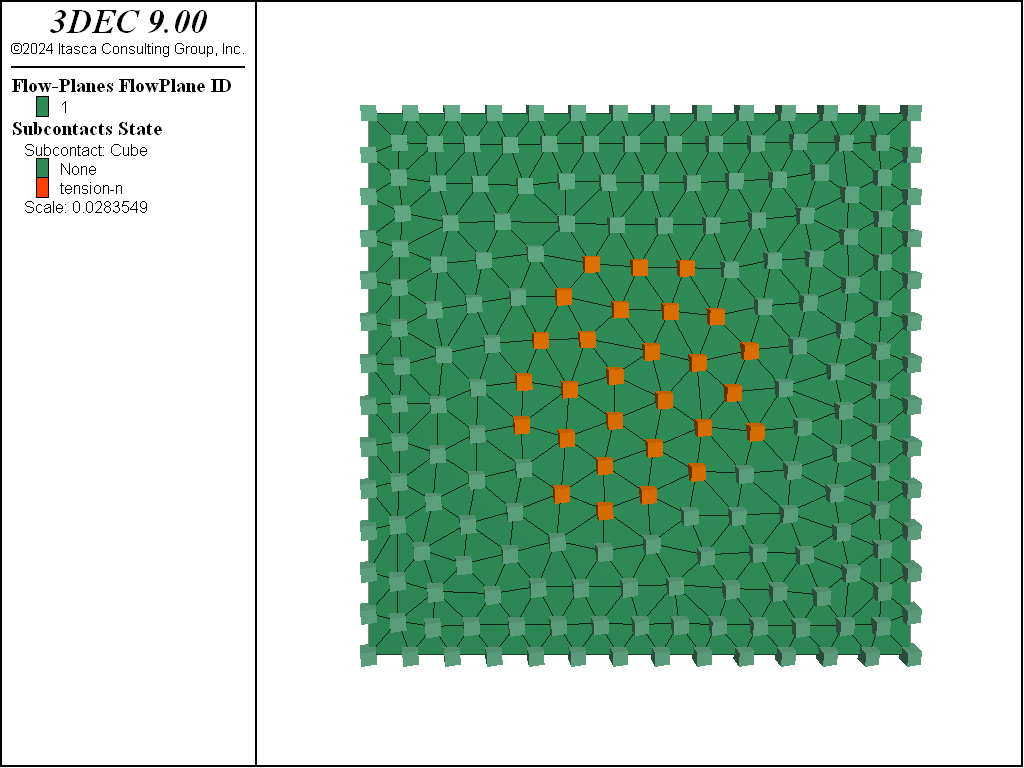
../../../../../_images/dfn-subcontacts-start.png — Figure 17: State of sub-contacts prior to injection.

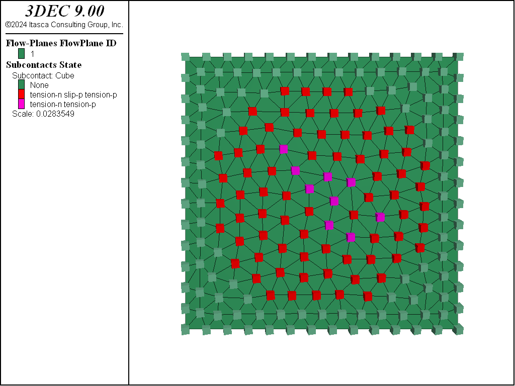
../../../../../_images/dfn-subcontacts-end.png — Figure 18: State of sub-contacts after 17 ms of injection.

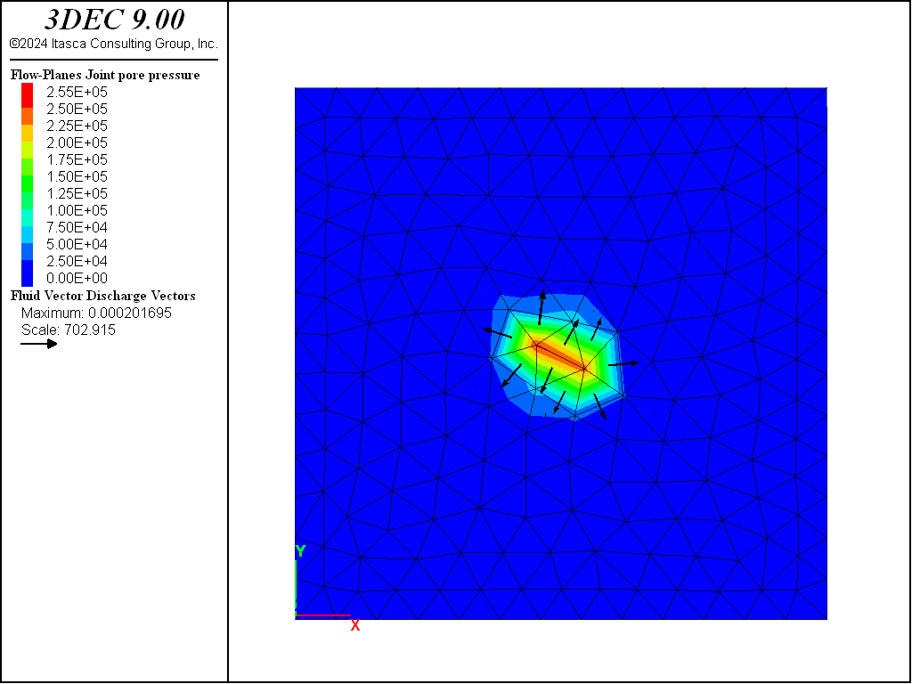
../../../../../_images/dfn-pressure.png — Figure 19: Pressures and discharge vectors after 17 ms of injection.

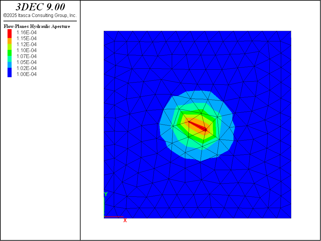
../../../../../_images/dfn-aperture.png — Figure 20: Joint aperture after 17 ms of injection.

Geometrical and Topological Model of a Fractured Rock Mass

Introduction

As previously discussed, in 3DEC the problem of fluid flow in rock masses is simplified to fluid flow through a network of fractures which are formed by joints separating the blocks. 3DEC model geometry is a simplified form of the internal structure of the rock, which is often very complex. In 3DEC, rock joints are assumed to be planar. The assumption of planarity (which is often not far from reality) considerably simplifies both the geometrical representation of the solid blocks and their geometrical interaction. Also in 3DEC, joints always extend to the boundaries of the block. Joints in a real rock mass are of finite size and usually elliptical in overall shape in the plane of the joint. In order to avoid creating partially fractured rock blocks, joints in the 3DEC model are assumed to be infinite, or to end exactly in the plane of another joint. The consequence of this assumption is that, after “cutting” the solid with joints, the model consists of convex polyhedral only. A possible method to simulate finite joints is described in Representation of a DFN for Fluid Flow Simulations.

3DEC Geometrical Entities

The geometries of rock blocks and fractures are represented in 3DEC by a number of simple geometric elements as described below.

3DEC blocks, which are equivalent to intact rock pieces, can only be convex polyhedra. Each surface of the block is a planar polygon, referred to as a face. Edges are the lines formed by intersection of two faces, and vertices are points formed by intersection of two lines. The basic geometric elements of block geometry are face (F), edge (E), and vertex (V).

The flow plane is the major geometrical element of the flow model. A flow plane is a two-dimensional surface (plane) in which flow is occurring through its thickness. (The equations of fluid flow are integrated over the thickness or aperture of the thin, planar interface.) The flow plane is the element of the 3DEC fluid flow data structure that corresponds to the face-to-face contact between two polyhedral blocks in the solid model (see Figure 4). Note that in 3DEC, contacts are relevant to the data structure for the solid phase calculation. In other words, the existence of two geometric entities of a flow plane and a face-to-face contact is not stemming from physical differences, but corresponds to the fact that it is preferable to keep the information and calculation corresponding to fluid and solid phase in two different data structures.

Flow planes are planar polygons since solid blocks are polyhedra with planar faces. Flow planes are connected along the edges, which are straight line segments. More than two flow planes can be connected along the same line. The line of connection between flow planes is called a flow pipe.

Fluid Flow Data Structure

The geometric elements of the flow model are:

flow plane — a planar polygon corresponding to a face-to-face contact between solid blocks
flow plane zone — a triangular discretization element of the flow plane
flow plane vertex — vertex of a flow plane zone, generally corresponding to a sub-contact between solid blocks
flow plane edge — a straight line that defines each segment on the periphery of a flow plane
flow plane edge segment — a subsegment of the flow plane edge
flow pipe — the intersection between one or more flow planes
flow pipe vertex — the vertex (end) of the flow pipe
flow pipe segment — subsegment of the flow pipe
flow knot — the same as a flow plane vertex except along the flow plane intersects, in which case one flow knot corresponds to two or more co-locational flow plane vertices from the intersecting flow planes. The flow knot stores the fluid pressures.

A graphical representation of some of these elements is shown in Figure 21.

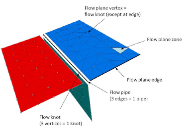
../../../../../_images/jointflow-structures.png — Figure 21: Flow structures for the intersection of three flow planes. The flow planes are actually connected but have been exploded for visualization.

The hierarchical and adjacency relations between elements in the data structure in both directions are shown in Figure 22. In this figure, vertical arrows indicate hierarchical relations, while horizontal arrows indicate adjacency relations. The dashed arrow is a pointer to the list (or loop) of the indicated elements.

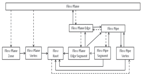
../../../../../_images/jointflow-links.png — Figure 22: Links in the data structure of the geometrical representation of the flow model.

Accessing Flow Plane Data

It is possible to loop through flow planes, flow plane vertices, flow plane zones or flow knots using loop foreach. An examle is shown in “get_pressures.fis”. In addition, a pointer to a single flow knot closest to some location can be obtained with the flowknotknot.near function. As shown in Figure 22, the flow plane is at the top of the flow structure hierarchy. While it is possible to loop through all flow plane zones or all flow plane vertices in the entire model using loop foreach, it is also possible to loop through all flow plane zones or flow plane vertices for a particular flow plane as shown in Example “flowzones.fis”.

In Figure 22, a dotted arrow indicates that the higher structure contains a pointer to a linked list of the lower structures (e.g., the flow plane contains a pointer to a linked list of flow plane zones). A solid arrow indicates a pointer to a single instance of the corresponding object (e.g., a flow plane edge contains a pointer to its flow plane). Please note the following exceptions:

Each flow plane points to the flow-plane edge list, which is a doubly linked list of flow-plane edges. The double-linked data structure allows traversal of the loop in both directions. This is essentially an infinite loop in which the last element links to the first element. Therefore, the user must be careful when looping through flow edges as shown in Example “test_pipe.fis”.
A flow pipe points to two flow pipe vertices representing the end points of the pipe.
A flow pipe segment points to two flow knots; one on each end of the segment.

Three examples are shown below. Example “get_pressures.fis” assumes there is a flow plane that contains a line along the \(x\)-axis. The pressures at flow knots along this line are printed out.

“flowzones.fis” shows how to loop through the flow zones associated with a particular flow plane.

“test_pipe.fis” outputs the coordinates of all of the flow pipe vertices. This example requires “FLOW.FIN”. Note that there may be some duplication since it loops through all of the flow plane edges to get the flow pipes. When there are intersecting flow planes, two or more flow plane edges will point to the same flow pipe Figure 21.

get_pressures.fis

; Function to print out pressures along x-axis
fish define get_pressures
    ; loop through flow knots
    loop foreach local knot flowknot.list
      local coord = flowknot.pos(knot)
      if math.abs(comp.z(coord)) < 0.01
        if math.abs(comp.y(coord)) < 0.01        
          local pressure_ = flowknot.pp(knot)
          local status = io.out('x: ' + string(comp.x(coord)) + ...
                                ' pp: ' + string(pressure_))
        endif
      endif
  end_loop
end

flowzones.fis

; Function to print out flow zone centroids for flow plane id 1
fish define get_flowzones
    ; loop through flow planes
    loop foreach local fp flowplane.list
      if flowplane.id(fp) = 2
        ; loop through all flow zones in this flowplane
        loop foreach local fz flowplane.zonelist(fp)        
          local status = io.out(string(flowplane.zone.pos(fz)))
        end_loop
      endif
    end_loop
end

test_pipe.fis

;
; Function to print out coordinates of flow pipe vertices
program call 'FLOW.FIN'
fish define test_pipe
  loop foreach fp flowplane.list
    local status = io.out('flow plane: '+string(fp))
    
    ; get index of flow plane for direct memory access
    local fp_index = flowplane.index(fp)
    
    local fpe_start = memory.fortran.index(fp_index+$klcor) ; flow plane edge
    local fpe = fpe_start
    loop while fpe # 0
      status = io.out(' flow plane edge '+string(fpe))
      local fpp = memory.fortran.index(fpe+$kpip) ; flow pipe
      status = io.out('  flow pipe: '+string(fpp))
      
      if fpp # index(9999) ; joined
      
        local fppv_left = memory.fortran.index(fpp+$kpleft)
        local fppv_right = memory.fortran.index(fpp+$kpright)
      
        local outstring = '   left vertex: ' + ...
                          string(memory.fortran.float(fppv_left+$kxyz))
        outstring = outstring + ',' + ...
                    string(memory.fortran.float(fppv_left+$kxyz+1))
        outstring = outstring + ',' + ...
                    string(memory.fortran.float(fppv_left+$kxyz+2))

        status = io.out(outstring)

        outstring = '   right vertex: ' + ...
                    string(memory.fortran.float(fppv_right+$kxyz))
        outstring = outstring + ',' + ...
                    string(memory.fortran.float(fppv_right+$kxyz+1))
        outstring = outstring + ',' + ...
                    string(memory.fortran.float(fppv_right+$kxyz+2))

        status = io.out(outstring)
      end_if
      fpe = memory.fortran.index(fpe + $knfe)
      if fpe = fpe_start
        exit loop
      end_if
    end_loop
  end_loop
end

Links between the Solid and Flow Models

The link between fluid flow data structure and the solid model is made through relations between:

The flow plane and the corresponding face-to-face contact of the solid blocks. The flow plane is accessed from the contact using the function block.contact.flowplane, and the contact is accessed from the flow plane using flowplane.contact.
The flowplane vertex and the corresponding sub-contact between solid blocks. Each sub-contact that does not lie on the edge of a plane contains a link to a flow plane vertex via block.subcontact.flowplane.vertex. Each flow plane vertex that is not on the edge of the flow plane also contains a link to the corresponding sub-contact via flowplane.vertex.subcontact1. In some cases, for the flow plane vertices on the flow plane edges, a single flow plane vertex will be between two sub-contacts, in which case the second sub-contact is given by flowplane.vertex.subcontact2, and the weights assigned to each sub-contact are given by flowplane.vertex.weight1 and flowplane.vertex.weight2.

Generation of Geometry of the Flow Model

The geometry of the flow model is generated automatically as a function of the geometry of the solid model (i.e., the shape of the solid blocks and the topological relations between the solid blocks). Therefore, no interaction with user is required. The fluid data structure is created mostly for computational reasons. In reality, flow paths are fractures which are defined by openings between blocks.

Gas Flow

Transient flow of a compressible gas through joints can also be simulated in 3DEC. The flow algorithm is based upon the algorithm used to model compressible flow of a fluid, with the following modifications. Modeling the flow of a gas requires consideration of the strong density dependence on pressure, which can usually be neglected when dealing with slightly compressible fluids, as is currently done in 3DEC.

For an ideal gas, we can consider the flow under isothermal conditions, for which

(23)\[\rho = B p\]

and adiabatic flow, for which

(24)\[\rho = B p^{\alpha}\]

where \(\rho\) is density, \(p\) is pressure, and \(B\) and \(\alpha\) are constants (see Chan et al. 1993). The \(B\) and \(\alpha\) constants are set in 3DEC with the command block fluid gas using keywords constant and \(alpha\) respectively.

As a consequence, the gas bulk modulus is also a function of pressure. In the isothermal case, we have, from Equation (23), the bulk modulus given by

(25)\[K_w = p\]

In the adiabatic case, it is

(26)\[K_w = {p \alpha}\]

The dependence of density on pressure requires that the spatial variation of density be taken into account in the fluid mass balance

(27)\[{\partial (n \rho) \over \partial t} + \nabla (\rho q) = 0\]

where \(n\) is the porosity. In contrast with the existing logic in 3DEC for slightly compressible fluids, the analysis of gas flowrequires the consideration of the convective terms, resulting from the density gradients in the second term of Equation (27).

Implementation

The modeling of fluid flow in 3DEC discontinuities is based on a discretization of the flow plane into a mesh of triangular flow zones, inside of which the pressure is assumed to vary linearly, and flow rates are assumed uniform. The flow mass balance is established at the flow plane vertices (nodes), considering the contribution from all the zones that contain the node. The update of the nodal pressure at every timestep may be expressed as

(28)\[p_{new} = p_{old} + K_g {1 \over V} \sum_{i} q_i {\rho_{im} \over \rho} \Delta t - K_g {\Delta V \over V}\]

The summation extends to all the triangular flow zones that include the node. The density of the triangular zone is taken as the average of the densities of the 3 nodes

(29)\[\rho_{im} = {{\rho_{i1} + \rho_{i3}} \over 3}\]

In Equation (28), the factor given by the ratio of the element mean density \(\rho_{im}\) and the old domain density \(\rho\) accounts for the spatial variation of the gas density, and is absent in the case of water flow. Density and bulk modulus for each domain are updated as a function of domain pressure, according to Equations (23) to (26).

Example

Chan et al. (1993) present the solution for a transient one-dimensional gas flow problem: the time evolution of the pressure of an ideal gas draining from a joint into a cavity. The problem conditions involve one-dimensional flow along the joint at constant volume in a semi-infinite domain. At \(x\) = 0, the gas pressure \(p\) = 0, and at \(x = \infty\), the gas pressure is set to \(p_1\).

The authors present both an approximate analytical solution and an empirical fit to a numerical solution obtained with an implicit time-marching scheme. They derive an approximate analytical solution for gas pressure along the joint:

(30)\[{\Psi \simeq 1 - exp(-\xi/\sqrt{2} -\xi^2/4})\]

They also present an empirical fit to a numerical solution:

(31)\[{\Psi = 1 - e^{-(0.625\xi+0.186\xi^2)}}\]

In Equations (30) and (31), dimensionless parameters \(\Psi = p^2 / p_1^2\), and \(\xi = \sqrt{{(\nu n x^2)} / {(t k p_1)}}\), where \(\nu\) is the shear viscosity of the gas, \(n\) is porosity, \(k\) is permeability, and \(t\) is time. The solutions are converted to a FISH function with results written to tables for comparison to 3DEC results. This FISH function, ppan, is listed below.

Analytical solution and empirical fit for 1D gas flow

The 3DEC model has a joint 100 m long in \(x\), with 10 blocks and 100 zones. The width (in \(y\)) is 1 m. At \(x\) = 0, pressure is fixed zero. At \(x\) = 100, the pressure is fixed at \(p_1\) = 1 MPa. The problem parameters are \(k\) = 10⁹, \(v\) = 10^-12, and \(n\) = 10^-4.

The 3DEC data file is listed in “gas_flow.dat”. A comparison of the 3DEC results to the analytical solution (Equation (30)) and the empirical fit (Equation (31)) at time = 0.5 is shown in Figure 23, and at time = 2.0 in Figure 24.

gas_flow.dat

; gas flow 1D test problem, solution by Chan et al. 1993
model new
model configure fluid
model large-strain off
;
block create brick 0 100 0 1 0 1
block create brick 0 100 0 1 -1 0
block densify segments 10 1 1 join

block zone generate edgelength 1.01
block zone cmodel assign elastic
; units in MPa
block zone property density 0.0027 young 1.0 poisson 0.2 

block contact jmodel assign elastic
block contact property stiffness-normal 1 stiffness-shear 1 
;
block fluid property bulk 1 density 1e-6 viscosity 0.0833e-9

flowplane vertex property aperture-initial 1e-4 aperture-minimum 0.5e-4 ...
                                                aperture-maximum 5e-4 
;
block insitu stress -1e-6 -1e-6 -1e-6 0 0 0 nodisplacements
block insitu pore-pressure 1
;
; gas flow
block fluid gas active on
block fluid gas alpha 1.0
block fluid gas constant 1.0
block fluid gas bulk-minimum 0.001
block fluid gas density-minimum 1e-6
;
block gridpoint apply velocity 0 0 0 range position-x 0 100
;
flowknot apply pore-pressure 0.0 range position-x 0
flowknot apply pore-pressure 1.0 range position-x 100
;
model history fluid time-total
flowknot history pore-pressure position 0.5 0 0
flowknot history pore-pressure position 1.5 0 0
flowknot history pore-pressure position 4.5 0 0
flowknot history pore-pressure position 8.5 0 0
flowknot history pore-pressure position 9.5 0 0

model fluid active on
model mechanical active off
;
program call 'gas_fish.fis'
[ppan]
[pp1dini]
;
model solve fluid time-total 0.5
[getpp1d(3)] ; 3DEC results in table '3'
table '3' label '3DEC - 0.5 s'
table '8' label 'Analytical - 0.5 s'
table '10' label 'Empirical - 0.5 s'
;
model solve fluid time-total 2.0
[getpp1d(4)] ; 3DECresults in table '4'
table '4' label '3DEC - 2 s'
table '9' label 'Analytical - 2 s'
table '11' label 'Empirical - 2 s'
;
;

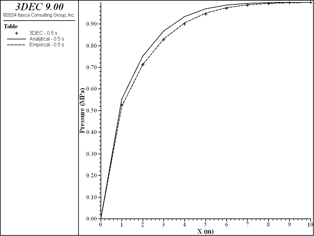
../../../../../_images/gas-t05.png — Figure 23: Gas pressures along the joint between \(x\) =0 and \(x\) =10 at \(t\) =0.5 s.

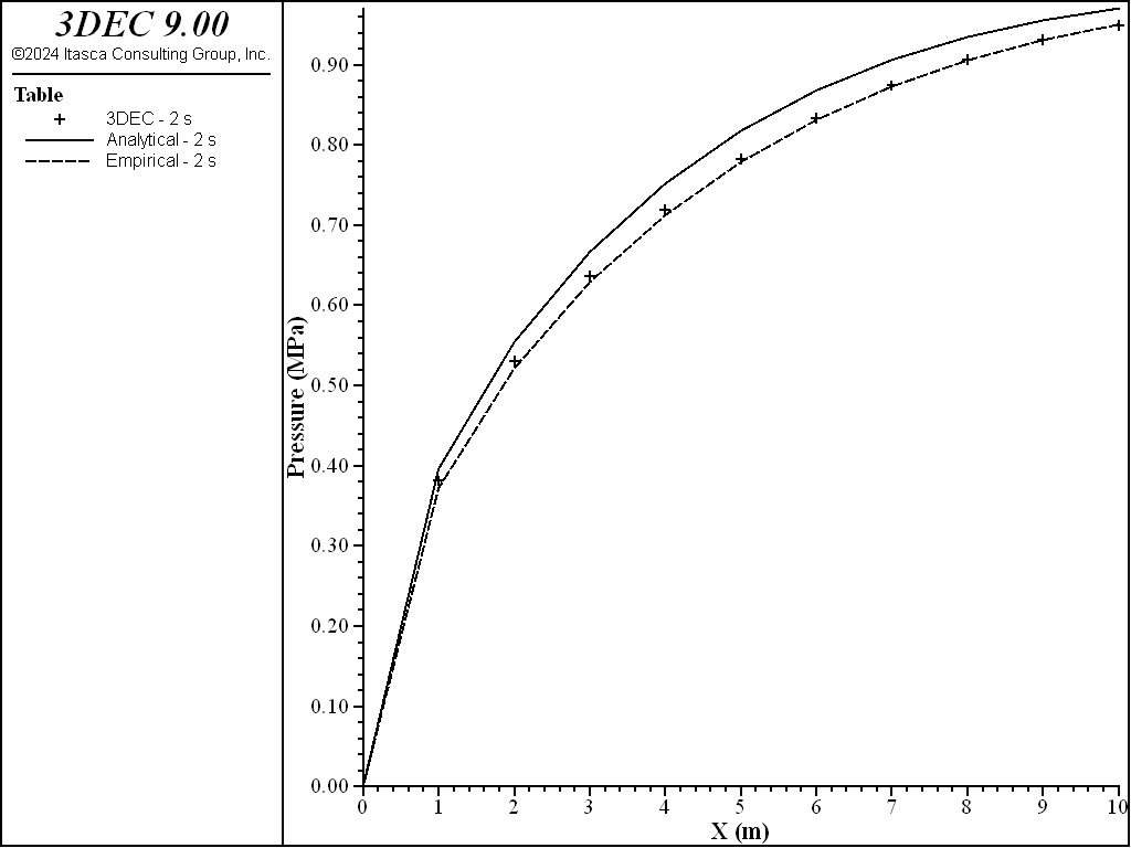
../../../../../_images/gas-t2.png — Figure 24: Gas pressures along the joint between \(x\) =0 and \(x\) =10 at \(t\) =2.0 s.

Fluid Discharge and Velocity

The rate of fluid flow in a joint can be plotted through Fluid Vectors / Discharge or Fluid Vectors / Velocity. Similarly, these quantities can be accessed by the FISH functions flowplane.zone.discharge and flowplane.zone.velocity. The discussion below describes how these values are calculated.

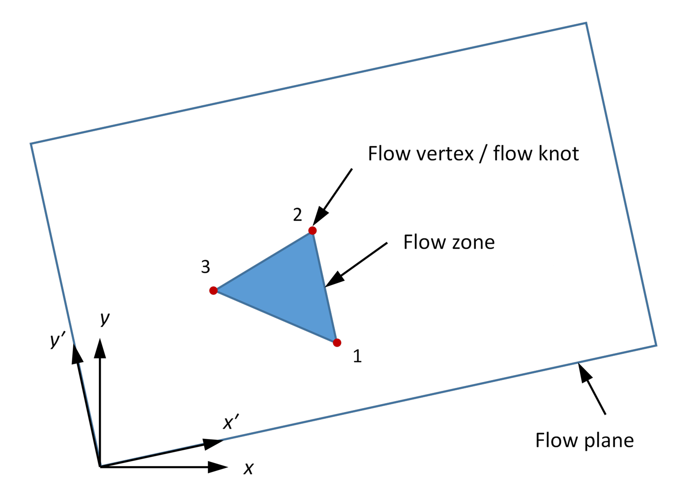
../../../../../_images/flowzone-geom.png — Figure 25: Geometry of a flow zone.

Given a flow zone with three vertices Figure 25, a pore pressure vector can be constructed that removes the effect of gravity:

(32)\[p_i = pp_i - \rho_f {\bf g \cdot x_i}\]

Where \(pp_i\) is the pore pressure at a flow knot \(i\), \(\rho_f\) is the density of the fluid, \(\bf{g}\) is the gravity vector and \(\bf{x_i}\) is the position of the flow knot in global coordinates. For the purposes of this discussion, it is assumed that there is one flow knot per flow vertex and that they are coincident.

A gradient can then be calculated by:

(33)\[{\bf \nabla x} = -{1 \over 2A} \left [\matrix{ y'_2 - y'_3 & y'_3 - y'_1 & y'_1 - y'_2 \cr x'_2 - x'_3 & x'_3 - x'_1 & x'_1 - x'_2 \cr }\right ]\]

Where \(A\) is the area of the flow zone, \(x'_i\) is the local \(x\)-coordinate of the \(i\)th flow knot and \(y'_i\) is the local \(y\)-coordinate of the \(i\)th flow knot.

The conductivity matrix is:

(34)\[{\bf k} = \left [\matrix{ {u^3_h \over 12v} & 0 \cr 0 & {u^3_h \over 12v} \cr }\right ]\]

where \(u_h\) is the hydraulic aperture and \(v\) is the fluid viscosity. The discharge in local coordinates is then

(35)\[\bf q_{local} = k \nabla xp\]

To get the discharge in global coordinates, the components of the 2D local discharge vector are just multiplied by the components of the 3D local axes:

(36)\[{\bf q} = {\bf x'} q_{local}^{x'} + {\bf y'} q_{local}^{y'}\]

Where \({\bf x'}\) and \({\bf y'}\) are the local axes vectors in global coordinates and \(q_{local}^{x'}\) and \(y' q_{local}^{y'}\) are the components of the discharge vector in local coordinates.

This results in a 3D vector with units of L²/T (e.g., m²/s in SI units). This vector is returned by the flowplane.zone.discharge FISH intrinsic.

The flow zone velocity can then be calculated by dividing by the average aperture of the zone:

(37)\[{\bf v} = {{\bf q} \over {(u_{h1} = u_{h2} + u_{h3})/3}}\]

Where \(u_{hi}\) is the hydraulic aperture associated with the \(i\)th flow zone vertex. This yields a value with units of L/T. This vector is returned by the flowplane.zone.velocity FISH intrinsic.

References

Alvarez, T. A., Jr., E. J. Cording and R. A. Milhail. “Hydromechanical Behavior of Rock Joints: A Re-interpretation of Published Experiments,” in Rock Mechanics (Proceedings of the 35th U.S. Symposium, University of Nevada, Reno, June 1995), pp. 665-671. J. J. K. Daemen and R. A. Schultz, eds. Rotterdam: A. A. Balkema (1995).

Bandis, S. C. Experimental Studies of Scale Effects on Shear Strength and Deformation of Rock Joints. Ph.D. Thesis, University of Leeds (1980).

Barton, N. R., S. C. Bandis and K. Bakhtar. “Strength, Deformation and Conductivity Coupling of Rock Joints,” Int. J. Rock Mech. Min. Sci. & Geomech. Abstr., 22(3), 121-140 (1985).

Batchelor, G. K. An Introduction to Fluid Dynamics. Cambridge University Press (1967).

Baumgart, B. G. “Winged Edge Polyhedron Representation,” Stanford Artificial Intelligence Project, Technical Report, Memo AIM-179, STAN-CS-320, Computer Science Department, School of Humanities and Science, Stanford University (1972).

Chan, D. Y. C., B. D. Hughes and L. Paterson. “Transient gas flow around boreholes,” Transport in Porous Media, 10, 137-152 (1993).

Detournay, E. “Hydraulic Conductivity of Closed Rock Fracture: an Experimental and Analytical Study,” in Proceedings of the 13th Canadian Rock Mechanics Symposium, pp. 168-173 (1980).

Iwai, K. Fundamental Studies of Fluid FlowThrough a SingleFracture. Ph.D. Thesis, University of California, Berkeley (1976).

Louis, C. “Rock Hydraulics,” in Rock Mechanics: Course Held at the Department of Mechanics of Solids, pp. 299-387. L. Muller, ed. Udine: Springer-Verlag (1974).

Robin, P.-Y. F. “Note on Effective Pressure,” J. Geophys. Res., 78(14), 2434-2437 (1973).

Walsh, J. B. “Effect of Pore Pressure and Confining Pressure on Fracture Permeability,” Int. J. Rock Mech. Min. Sci. & Geomech. Abstr., 18, 429-435 (1981).

Witherspoon, P. A., et al. “Validity of Cubic Law for Fluid Flow in a Deformable Rock Fracture,” Water Resources Res., 16(6), 1016-1024 (1980).

Endnote

⇄

⇐ Matrix Fluid Flow | Proppant ⇒

Was this helpful? ...

Updated: Nov 20, 2024