Nonlinear Joint Model In 3DEC

The Nonlinear model is the same as the Mohr-Coulomb Joint Model In 3DEC except that the normal and shear stiffness may depend on the normal stress as in the Continuously Yielding Joint Model In 3DEC. The tiffness behavior differs from the Continuously-Yielding Joint Model in that during unloading, the stiffness is constant and is equal to the stiffness at the point of unloading.

Formulations

The response to normal loading is expressed incrementally as

(1)\[Δ\sigma_n = k^{current}_n\ Δu_n\]

where the normal stiffness, \(k^{current}_n\), is given by

(2)\[k^{current}_n = k_n\ \sigma^{e_n}_n\]

representing the observed increase of stiffness with normal stress, where \(k_n\) and \(e_n\) are input model parameters.

If the normal stress descreases (becomes less compressive), then the normal stiffness is constant and equal to the normal stiffness at the start of unloading. The stiffness will remain constant as the joint is reloaded, until the main loading path is rejoined. This is illustrated in Figure 1.

A maximim and minimum value of normal stiffness may also be supplied by the user. If not provided, these will default to \(k_n\).

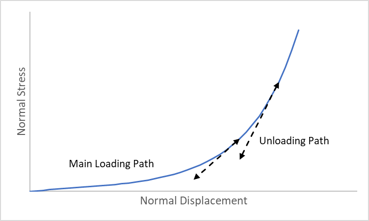
Figure 1: 3DEC Nonlinear joint normal stress versus normal displacement behavior.

The shear stiffness can also vary with normal stress. The relationship is essentially the same:

(3)\[k^{current}_s = k_s\ \sigma^{e_s}_n\]

where \(k_s\) and \(e_s\) are input model parameters. A maximim and minimum value of shear stiffness may also be supplied by the user. If not provided, these will default to \(k_s\).

Summary of Nonlinear Parameters

The model parameters associated with the nonlinear model are summarized in Table 1. The model is accessed in 3DEC with the block contact jmodel assign nonlinear command.

Table 1: Parameters associated with the Nonlinear joint model

Parameter	Description	Keyword
\(k_n\)	initial joint normal stiffness (STRESS/LENGTH)	stiffness-normal
\(k^{max}_n\)	maximum joint normal stiffness (STRESS/LENGTH). Defaults to k_n.	kn-maximum
\(k^{min}_n\)	minimum joint normal stiffness (STRESS/LENGTH). Defaults to k_n.	kn-minimum
\(k^{current}_n\)	current calculated joint normal stiffness (read only)	kn-current
\(e_n\)	joint normal stiffness exponent	exponent-normal
\(k_s\)	initial joint shear stiffness (STRESS/LENGTH)	stiffness-shear
\(k^{max}_s\)	maximum joint shear stiffness (STRESS/LENGTH). Defaults to k_s.	ks-maximum
\(k^{min}_s\)	minimum joint shear stiffness (STRESS/LENGTH). Defaults to k_s.	ks-minimum
\(k^{current}_s\)	current calculated joint shear stiffness (read only)	ks-current
\(e_s\)	joint shear stiffness exponent	exponent-shear
\(\phi\)	friction angle (DEGREES)	friction
\(\phi_{res}\)	residual friction angle (DEGREES). Defaults to phi.	friction-residual
\(c\)	cohesion (STRESS)	cohesion
\(c_{res}\)	residual cohesion (STRESS). Defaults to 0.	cohesion-residual
\(\psi\)	dilation angle (DEGREES)	dilation
\(u_{cs}\)	shear displacement at which dilation stops (LENGTH). Default is infinity	dilation-zero
\(T_f\)	tensile strength (STRESS)	tension
\(T_f^{res}\)	residual tensile strength (STRESS). Default is 0.	tension-residual

Example: Normal Loading

The following example illustrates the behavior with a simple test model. The problem applies a varying normal load to the top block of a two-block system.

To view this example in 3DEC, use the menu command Help -> Examples…. The data file used is shown at the end of this example.

The modeled joint is first subjected to an increasing normal load. This is followed to by an unload-reload excursion to test the functionality of the non-linear joint normal stiffness calculation. The shear stiffness is kept constant. Figure 2 shows the model; the joint is defined by one contact that is composed of 10 sub-contacts. The properties used in this test are:

Table 2: Nonlinear joint model properties for examples

Property Keyword	Param.	Description	Value
density	\(\rho\)	block mass density	2600 kg/m3
bulk	\(K\)	bulk modulus of block	4 GPa
shear	\(G\)	shear modulus of block	3 GPa
stiffness-normal	\(k_n\)	joint initial normal stiffness	10 GPa/m
stiffness-shear	\(k_s\)	joint shear stiffness	10 GPa/m
exponent-normal	\(e_n\)	joint normal stiffness exponent	1.1
kn-maximum	\(k^{max}_n\)	maximum joint normal stiffness	1000 GPa/m
friction	\(\phi\)	joint intrinsic friction angle	30º
roughness	\(R\)	joint roughness parameter	0.1 mm
dilation	\(\psi\)	dilation angle	15º

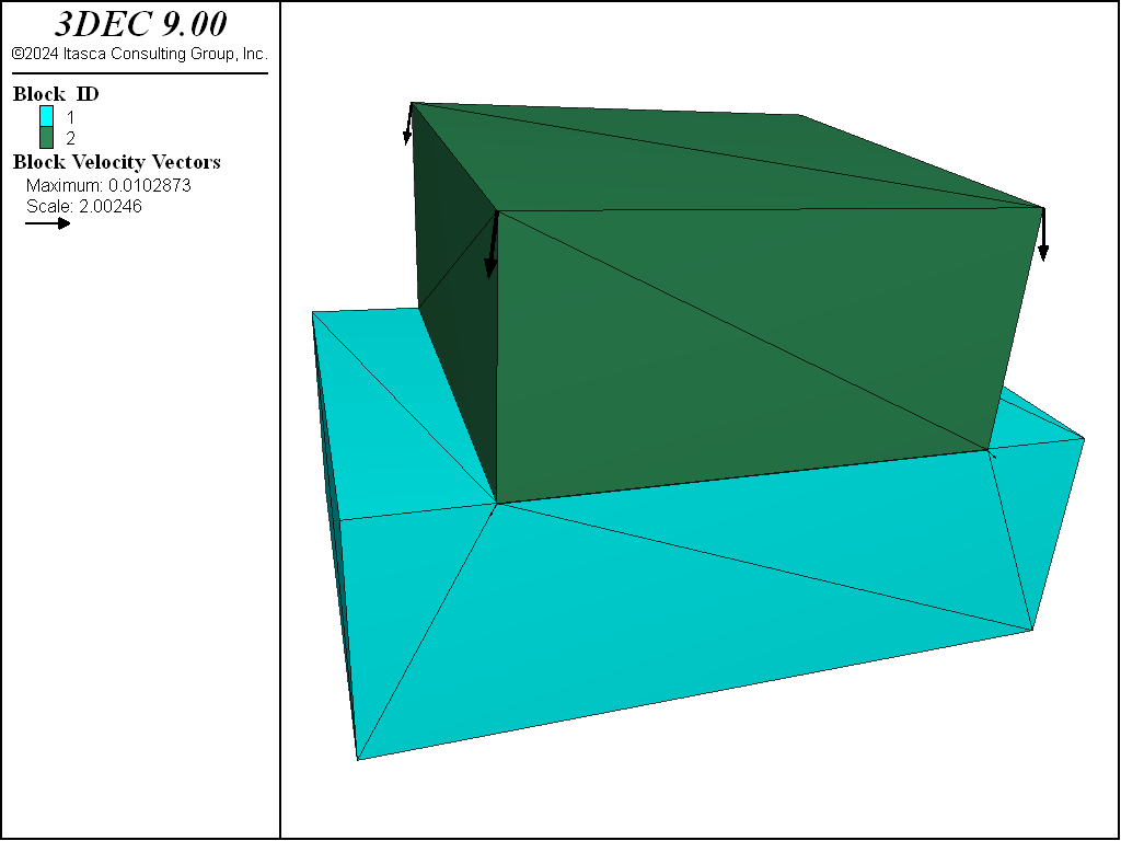
Figure 2: 3DEC model used to test nonlinear joint behavior.

A graph of normal stress verus normal dispacement during the first loading step is shown in Figure 3. Initially the line is linear with a slope equal to the input value of k_n. After about 0.15 mm of displacement, the stiffness increases (the line becomes steeper).

The joint is then unloaded and the response is shown in Figure 4. The stiffness remains constant and equal to the tangent stiffness at the start of unloading.

Finally, the joint is reloaded (Figure 5). The normal stress increases back up along the unload line until rejoining the main loading curve, at which time the stiffness starts to increase again.

The change in normal stiffness throughout the test is shown in Figure 6.

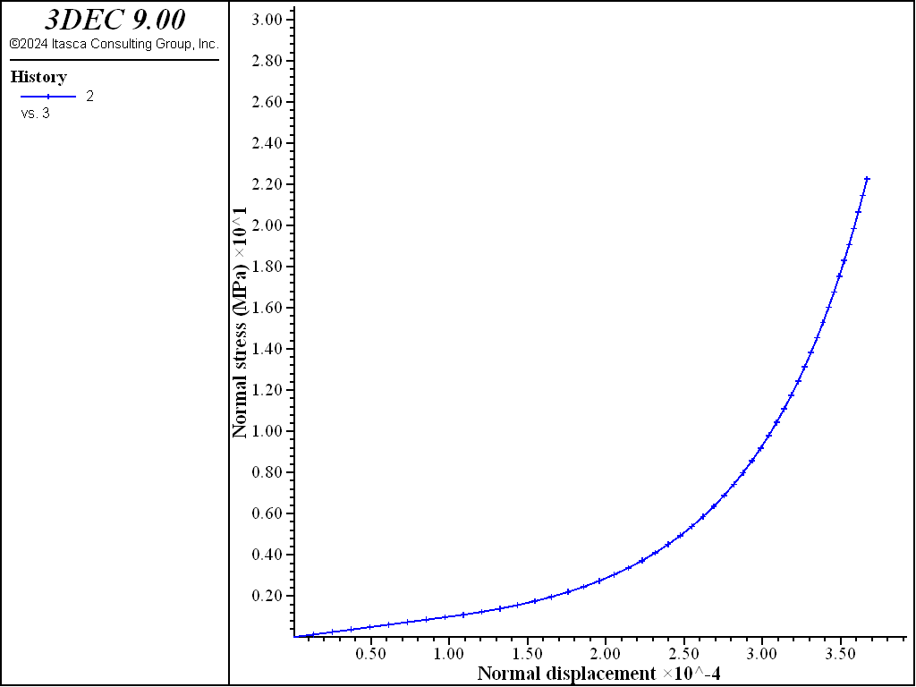
Figure 3: Normal stress vs. normal displacement during normal loading of the joint.

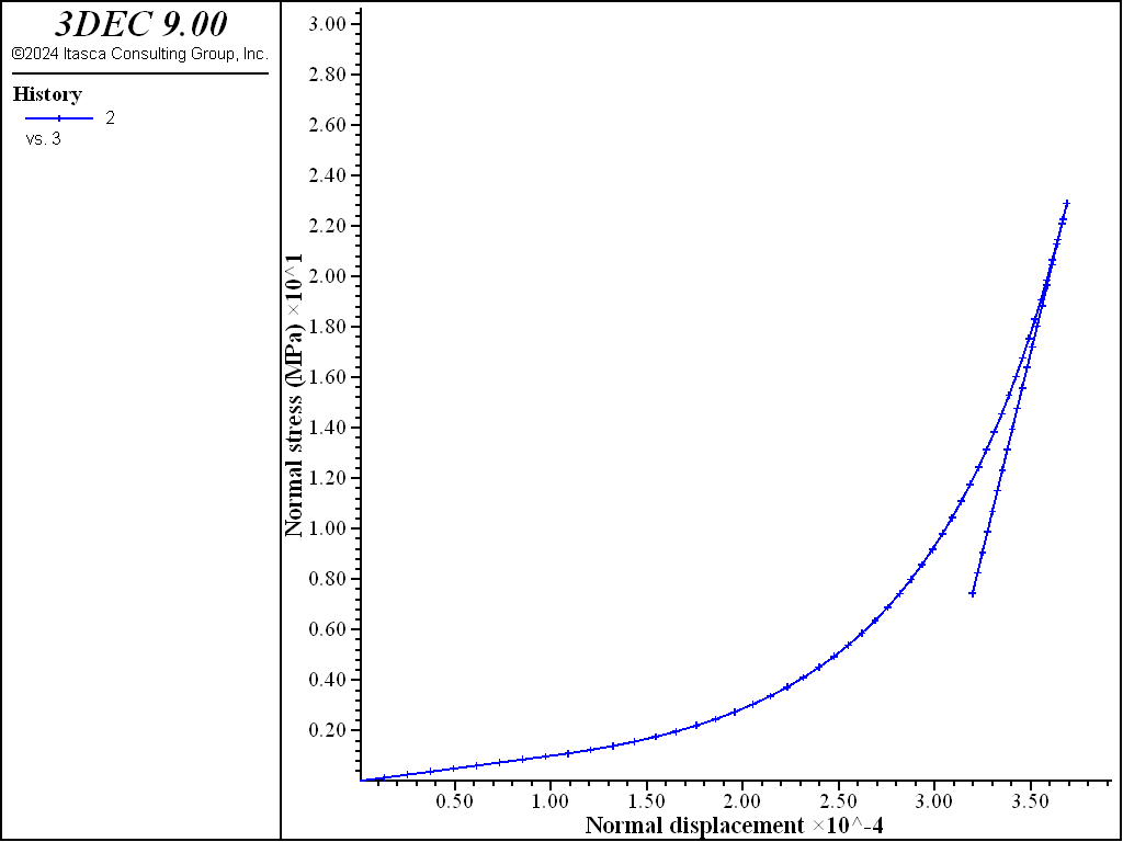
Figure 4: Normal stress vs. normal displacement during after unloading.

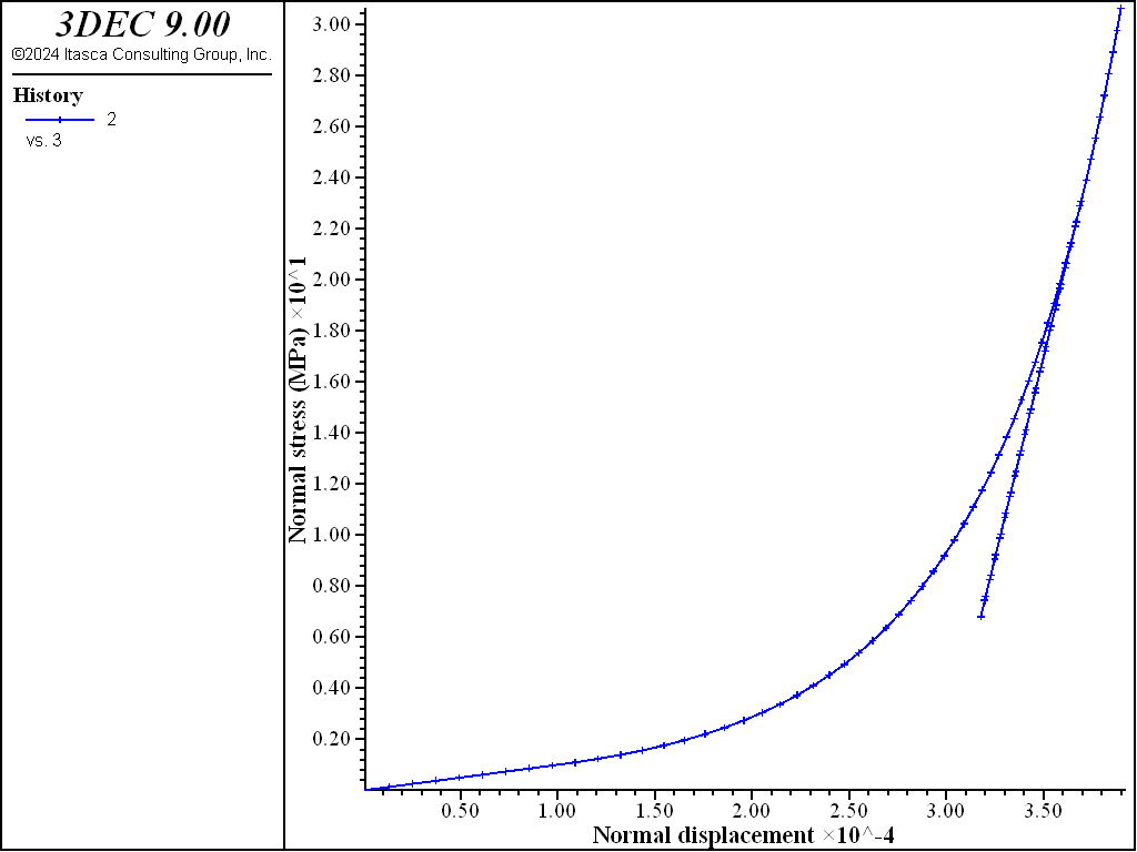
Figure 5: Normal stress vs. normal displacement after reloading.

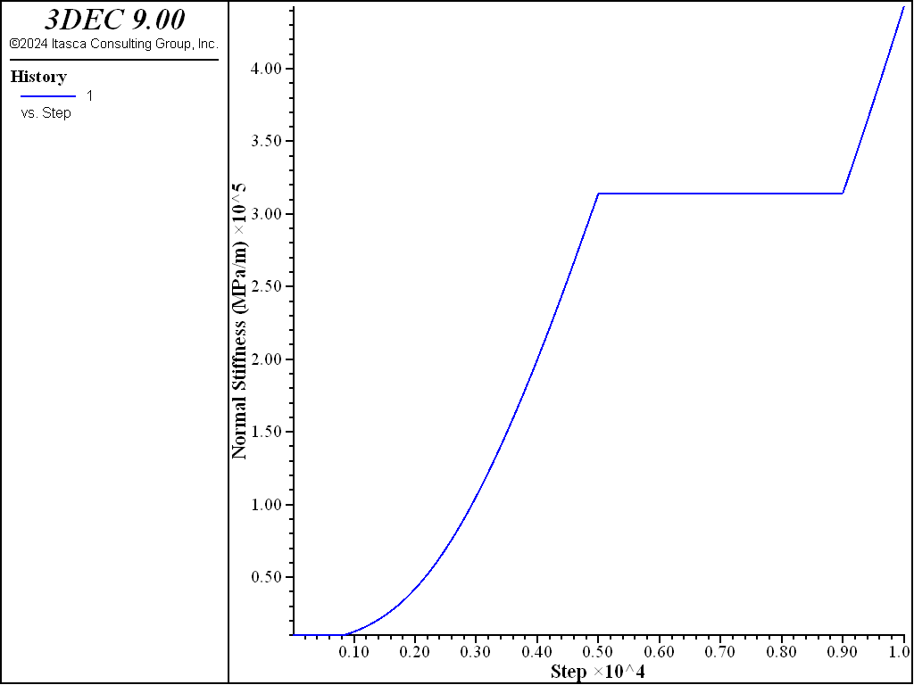
Figure 6: Change in normal stiffness during the load-unload-reload cycle.

Data File

compression.dat

model new
model large-strain on
;
block create brick  -0.15,0.15 -0.10,0.10 -0.10,0
block create brick  -0.10,0.10  -0.10,0.10 0,0.10

block zone generate edgelength  0.2

block zone cmodel assign elastic
block zone property  density=0.0026  bulk=4000   shear=3000
;
 ;  Nonlinear slip model
block contact jmodel assign nonlinear
block contact property stiffness-normal=1e4 stiffness-shear=1e4  ...
                   friction=30.0 exponent-normal 1.1 kn-maximum 1e6
;
block contact material-table default jmodel nonlinear
block contact material-table default property stiffness-normal=1e4  ...
                                          stiffness-shear=1e4  ...
                                          friction=30.0 ...
                                          exponent-normal 1.1 ...
                                          kn-maximum 1e6 ...
                                          dilation 15

block hide range position-z 0 1
block gridpoint apply velocity 0 0 0 range position-z -1 0.1
block hide off

;; test insitu
;block insitu stress 0 0 -10 0 0 0
;
; normal load
block gridpoint group 'top' range position-z 0.1
block gridpoint apply velocity-z -0.01 range group 'top'

fish define kn
  cx = block.subcontact.near(-0.1,-0.1,0)
  kn = block.subcontact.prop(cx,'kn-current')
end

fish history kn
block contact history stress-normal position -0.1 -0.1 0
block contact history displacement-normal position -0.1 -0.1 0

;
model cycle 5000

model save 'load'

; now unload
block gridpoint apply velocity-z 0.01 range group 'top'

model cycle 2000

; test save/restore
model save 'unload'
model restore 'unload'

; now reload
block gridpoint apply velocity-z -0.01 range group 'top'

model cycle 3000

model save 'reload'

Example: Shear Loading

The same model as above is loaded in shear. An insitu normal stress of 10 MPa is first applied. This results in an initial normal stiffness of 31.6 GPa/m. The top of the model is fixed during shear loading. This causes the normal stress on the joint to increase once dilation starts. This increase in normal stress causes the normal stiffness to increase. A plot of shear stress verusus shear displacement is shown in Figure 7 and the variation in normal stiffness is shown in Figure 8

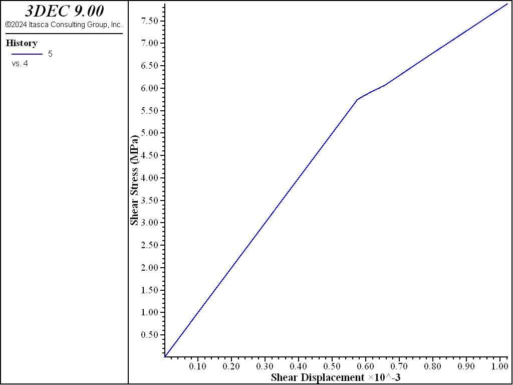
Figure 7: Shear stress versus shear displacement in the shearing test.

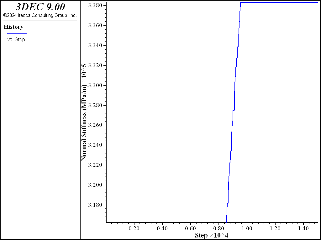
Figure 8: Normal stiffness in the shearing test.

Data File

shear.dat

model new
model large-strain on
;
block create brick  -0.15,0.15 -0.10,0.10 -0.10,0
block create brick  -0.10,0.10  -0.10,0.10 0,0.10

block zone generate edgelength  0.2

block zone cmodel assign elastic
block zone property  density=0.0026  bulk=4000   shear=3000
;
 ;  Nonlinear slip model
block contact jmodel assign nonlinear
block contact property stiffness-normal=1e4 stiffness-shear=1e4  ...
                   exponent-normal 1.5 kn-maximum 1e6 ...
                   friction=30.0 dilation 15 

block contact material-table default jmodel nonlinear
block contact material-table default property stiffness-normal=1e4  ...
                                     stiffness-shear=1e4  ...
                                     exponent-normal 1.5 kn-maximum 1e6 ...
                                     friction=30.0 dilation 15 

block hide range position-z 0 1
block gridpoint apply velocity 0 0 0 range position-z -1 0.1
block hide off
;
; normal load
block insitu stress 0 0 -10  0 0 0 
block gridpoint apply velocity-z 0 range position-z 0.1
;
model solve
;
block contact reset displacement

; shear load
block hide range position-z -.1 0.0
block gridpoint apply  velocity-x=0.005 range position-z -.1 1.1
block gridpoint apply  velocity-y 0 range position-z -1 1
block hide off

fish define kn
  cx = block.subcontact.near(-0.1,-0.1,0)
  kn = block.subcontact.prop(cx,'kn-current')
end

fish history kn

block contact history stress-normal position -0.1 -0.1 0
block contact history displacement-normal position -0.1 -0.1 0

block contact history  displacement-shear position -0.1 -0.1 0
block contact history  stress-shear position -0.1 -0.1 0

model cycle 15000

model save 'shear'
program return

Example: Shear Loading with Non-linear Shear Stiffness

The model above is used but a changing normal stress is applied to the top boundary to observe how the shear stiffness is affected. An insitu normal stress of 1 MPa is first applied. This results in an initial shear stiffness of 10 GPa/m (the minimum). The joint is then sheared for 1000 steps. The normal stress is then increased in increments of 1 MPa with shearing after each normal stress change. This increase in normal stress causes the shear stiffness to increase. After 4000 steps, the normal stress is decreased and then increased again. The variation in shear stiffness is shown in Figure 9. You can see how the shear stiffness increases with each increase in normal stress, but between 4000 and 6000 steps, the shear stiffness doesn’t change as the joint expeirneces unloading and reloading. Finally, normal stiffness is increased further and the shear stiffness reaces its maximum value (100 GPa/m). A plot of shear stress verusus shear displacement is shown in Figure 10.

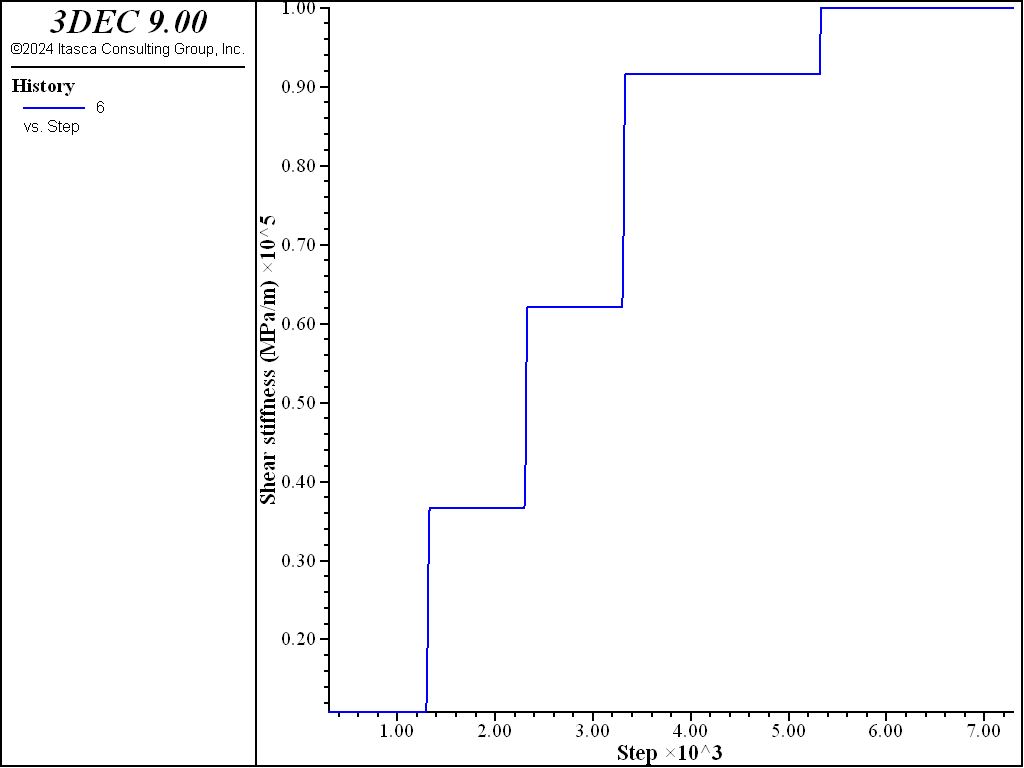
Figure 9: Shear stiffness in the second shearing test.

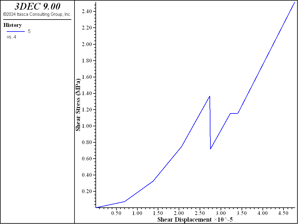
Figure 10: Shear stress versus shear displacement in the second shearing test.

Data File

shear2.dat

model new
model large-strain off
;
block create brick  -0.15,0.15 -0.10,0.10 -0.10,0
block create brick  -0.10,0.10  -0.10,0.10 0,0.10

block zone generate edgelength  0.2

block zone cmodel assign elastic
block zone property  density=0.0026  bulk=4000   shear=3000
;
 ;  Nonlinear slip model
block contact jmodel assign nonlinear
block contact property stiffness-normal=1e4 stiffness-shear=1e4  ...
                   exponent-shear 1.5 ks-maximum 1e5 ...
                   friction=30.0 dilation 15 

block hide range position-z 0 1
block gridpoint apply velocity 0 0 0 range position-z -1 0.1
block hide off
;
; normal load
block insitu stress 0 0 -1  0 0 0 
block face apply stress-zz -1 range position-z 0.1
;
model solve
;
block contact reset displacement

; shear load
block hide range position-z -.1 0.0
block gridpoint apply  velocity-x=0.0005 range position-z -.1 1.1
block gridpoint apply  velocity-y 0 range position-z -1 1
block hide off

fish define kn
  cx = block.subcontact.near(-0.1,-0.1,0)
  kn = block.subcontact.prop(cx,'kn-current')
  ks = block.subcontact.prop(cx,'ks-current')
end

fish history kn

block contact history stress-normal position -0.1 -0.1 0
block contact history displacement-normal position -0.1 -0.1 0

block contact history  displacement-shear position -0.1 -0.1 0
block contact history  stress-shear position -0.1 -0.1 0

fish history ks

model cycle 1000

block face apply stress-zz -1 range position-z 0.1  ; total = 2
model cycle 1000

block face apply stress-zz -1 range position-z 0.1 ; total = 3
model cycle 1000

block face apply stress-zz -1 range position-z 0.1 ; total = 4
model cycle 1000

; unload

block face apply stress-zz 2 range position-z 0.1
model cycle 1000

; reload

block face apply stress-zz -2 range position-z 0.1
model cycle 1000

; get to the max

block face apply stress-zz -5 range position-z 0.1 ; total = 5
model cycle 1000

model save 'shear'
program return

Properties

nonlinear

cohesion f

Joint cohesion.

cohesion-residual f

Residual joint cohesion.

dilation f

Joint dilation angle in degrees.

dilation-zero f

Shear displacement at which joint will cease to dilate.

exponent-normal f

Joint normal stiffness exponent

exponent-shear f

Joint shear stiffness exponent

friction f

Friction angle in degrees.

friction-residual f

Residual joint friction angle in degrees.

stiffness-normal f

Initial joint normal stiffness (stress / distance)

stiffness-shear f

Joint shear stiffness (stress / distance)

kn-current f

Current calculated joint normal stiffness (stress / distance) (read only)

kn-maximum f

Maximum joint normal stiffness (stress / distance)

kn-minimum f

Minimum joint normal stiffness (stress / distance)

ks-current f

Current calculated joint shear stiffness (stress / distance) (read only)

ks-maximum f

Maximum joint shear stiffness (stress / distance)

ks-minimum f

Minimum joint shear stiffness (stress / distance)

tension f

Tensile strength.

tension-residual f

Residual joint tensile strength.