Softening-Healing Mohr-Coulomb Joint Model In 3DEC

The Mohr-Coulomb joint model has the following deficiencies when used to model seismicity.

• The stress drop is instantaneous when slipping starts (shear strength drops instantaneously from a peak to a residual value). This means that all slip events are seismic (see Figure 1).

• Once slip has occurred, there is no way for the strength on the fault to recover back to the peak value. This means that stick-slip behavior is not possible.

Figure 1: (a) Stable response of a slip-weakening fault system in a stiff system; and (b) unstable response in a soft system (after Rice, 1983). The straight line represents the unloading of the system and the curved line represents unloading of the fault. In the stable case, the system unloads faster than the fault. The opposite is true for the unstable case.

Formulation

The Softening Healing Mohr-Coulomb model is based on the standard i Mohr-Coulomb model, with two additions.

• When the joint starts slipping, the shear strength evolves from the peak value to the residual value over a user-specified critical slip distance \(D_c\).

• When slipping stops, the shear strength recovers instantaneously to the peak value.

There is no softening or healing for the tensile forces. The tensile strength drops instantaneously when the strength is exceeded (no softening) and the tensile strength remains at the residual value (no healing).

For a non-slipping joint, the value of cohesion and friction are the peak values. When the strength is exceeded, the strength is a function of the slip distance. When the slip distance exceeds the critical slip distance, the residual values of cohesion and friction are used. Two formulations for the evolution of shear strength are provided.

Linear

For linear softening, the shear strength is calculated by:

(1)\[ \begin{align}\begin{aligned}S_F = S_F^{peak} = c + \sigma_n \tan\phi \; , \; u_s^p = 0\\S_F = S_F^{peak} - (S_F^{peak} - S_F^{resid}) \ast {u_s^p \over D_c } \; , \; 0 < u_s^p < D_c\\S_F = S_F^{resid} = c_{resid}+ \sigma_n \tan\phi_{resid} \; , \; u_s^p > D_c\end{aligned}\end{align} \]

where \(c\) is the cohesion, \(\sigma_n\) is the normal stress, \(\phi\) is the friction angle, \(c_{resid}\) is the residual cohesion, \(\phi_{resid}\) is the residual friction angle, \(D_c\) is the critical slip distance, and \(u_s^p\) is the plastic shear displacement (slip) since the start of slipping. When slipping stops, the shear strength returns instantaneously to the peak value and \(u_s^p\) is set back to 0.

An example of a subcontact with no cohesion is shown in Figure 2.

Figure 2: Shear stress versus shear displacement for a slipping joint with constant normal stress. The linear softening law is used.

Non-Linear

For non-linear softening, the shear strength is calculated by:

(2)\[ \begin{align}\begin{aligned}S_F = S_F^{peak} = c + \sigma_n \tan\phi \; , \; u_s^p = 0\\S_F = S_F^{resid} + (S_F^{peak} - S_F^{resid}) \ast {D_c^\alpha \over (D_c + u_s^p)^\alpha } \; , \; u_s^p > 0\end{aligned}\end{align} \]

where \(\alpha\) is an exponent (> 1) that dictates the severity of the strength drop (see Figure 3).

Figure 3: Shear stress versus shear displacement for a slipping joint with constant normal stress. The non-linear softening law is used.

Dilation (\(\psi\)) behaves in the same way as cohesion or friction. If a non-zero residual dilation is specified, the dilation varies according to the following equation for \(\alpha\) = 0 (linear):

(3)\[ \begin{align}\begin{aligned}\tan\psi = \tan\psi_{peak} - (\tan\psi_{peak} - \tan\psi_{resid}) \ast {u_s^p \over D_c } \; 0 < u_s^p < D_c\\\tan\psi = \tan\psi_{resid} \; , \; u_s^p > D_c\end{aligned}\end{align} \]

For the non-linear case, the dilation is given by:

(4)\[\tan\psi = \tan\psi_{resid} + (\tan\psi_{peak} - \tan\psi_{resid}) \ast {D_c^\alpha \over (D_c + u_s^p)^\alpha } \; , \; u_s^p > 0\]

If a value of \(\psi_{resid}\) is not provided, it defaults to \(\psi_{peak}\) .

Subcontact failure states are the same as for i Mohr-Coulomb Joint Model In 3DEC.

Summary of Softening-Healing Mohr-Coulomb Parameters

The model parameters associated with the sofdtening-healing mohr-coulomb model are summarized in Table 1. The model is accessed in 3DEC with the block contact jmodel assign softening-mohr command.

Table 1: Parameters associated with the Softening-Healing Mohr-Coulomb joint model

Parameter	Description	Keyword
\(k_n\)	joint normal stiffness (STRESS/LENGTH)	stiffness-normal
\(k_s\)	joint shear stiffness (STRESS/LENGTH)	stiffness-shear
\(\phi\)	friction angle (DEGREES)	friction
\(\phi_{res}\)	residual friction angle (DEGREES). Defaults to phi.	friction-residual
\(c\)	cohesion (STRESS)	cohesion
\(c_{res}\)	residual cohesion (STRESS). Defaults to 0.	cohesion-residual
\(\psi\)	dilation angle (DEGREES)	dilation
\(u_{cs}\)	shear displacement at which dilation stops (LENGTH). Default is infinity	dilation-zero
\(T_f\)	tensile strength (STRESS)	tension
\(T_f^{res}\)	residual tensile strength (STRESS). Default is 0.	tension-residual
\(D_c\)	critical slip distance (LENGTH)	dc
\(\alpha\)	exponent that dictates the severity of non-linear stress drop	alpha
	boolean to indicate if healing is on or off (default is on)	healing
\(\phi_{current}\)	current friction angle (DEGREES). Read only.	friction-current
\(u_s^p\)	plastic slip (LENGTH). Read only.	slip

Example

To view this example in 3DEC, use the menu command Help ► Examples…. Choose “3DEC/ Constitutive_Models/ SHMohr_Model” and select “shmohr.prj” to load. The data files used are shown at the end of this example.

A spring-slider problem is simulated with three blocks as shown in Figure 4. A normal stress of 1 MPa is applied to the top surface of the slider block. A velocity of 1 mm/s is applied to the right side of the system. The model is then run until one or more slip events occurs.

The test is a simulation of a direct shear test, which consists of a single horizontal joint that is first subjected to a normal confining stress, and then to a unidirectional shear displacement. Figure 5 shows the model; the joint is defined by one contact that is composed of 10 sub-contacts.

The following strength properties are assigned to the sliding joint.

Peak friction	\(\phi\)	25 degrees
Residual friction	\(\phi_{resid}\)	20 degrees
Critical slip distance	\(D_c\)	1 × 10-4, 1 × 10-5
Alpha exponent	\(\alpha\)	0 (linear)

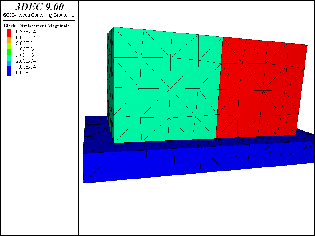
Figure 4: 3DEC Block configuration in the spring-slider test.

Plots of friction on the joint, and shear velocity versus shear displacement are shown for the different values of \(D_c\) in Figure 5 to Figure 8. Velocities are plotted with the same maximum in each plot to facilitate comparison. The effect of the softening is clear, and the higher velocities observed in the model with the lower value of \(D_c\) suggest a possible criterion for differentiating seismic and aseismic slip events.

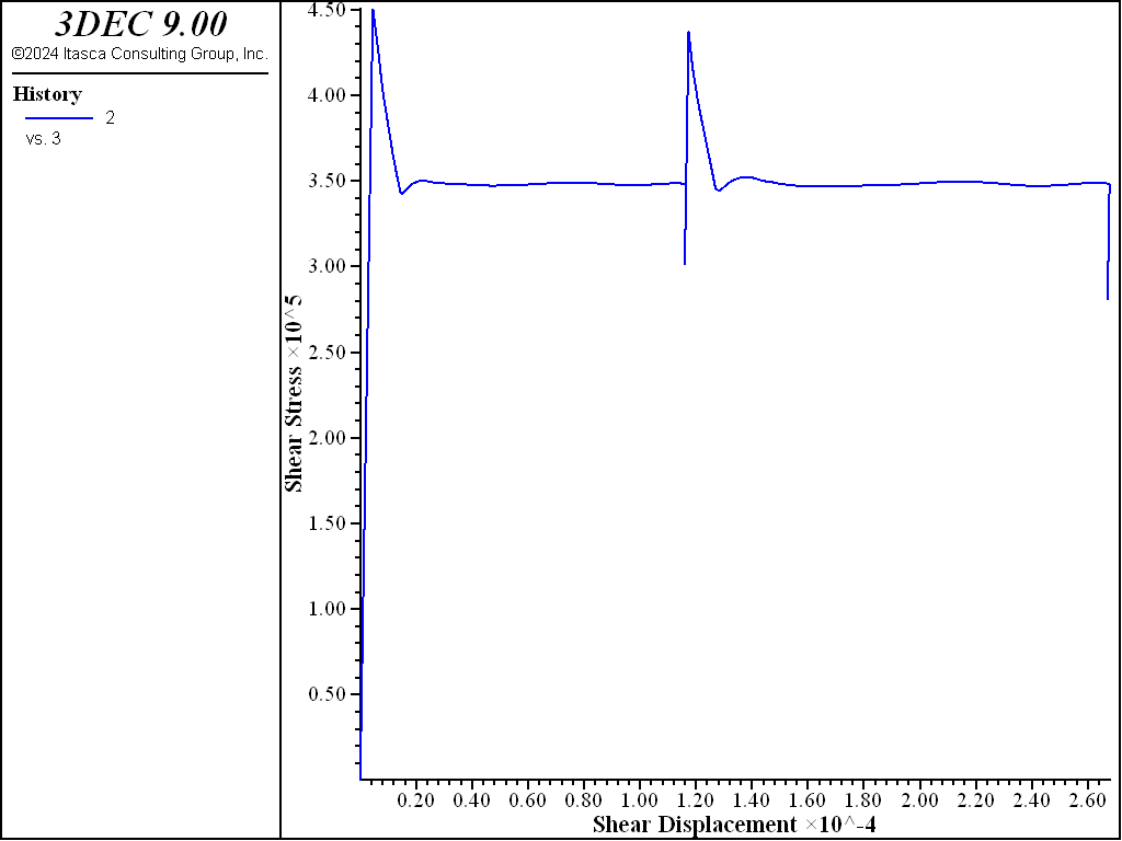
Figure 5: Average shear stress versus shear displacement in the Softening-Healing-Mohr-Coulomb joint model with \(D_c\) = 1e-5.

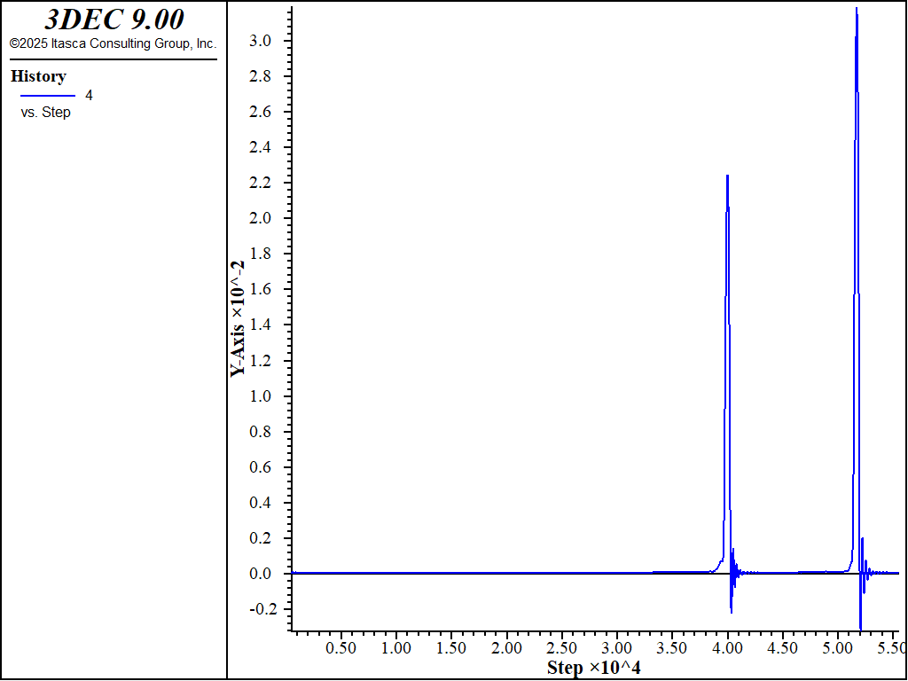
Figure 6: Shear velocity versus shear displacement in the Softening-Healing-Mohr-Coulomb joint model with \(D_c\) = 1e-5.

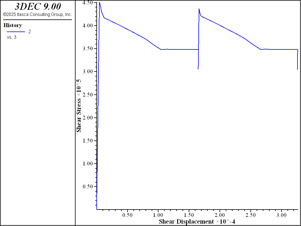
Figure 7: Average shear stress versus shear displacement in the Softening-Healing-Mohr-Coulomb joint model with \(D_c\) = 1e-4.

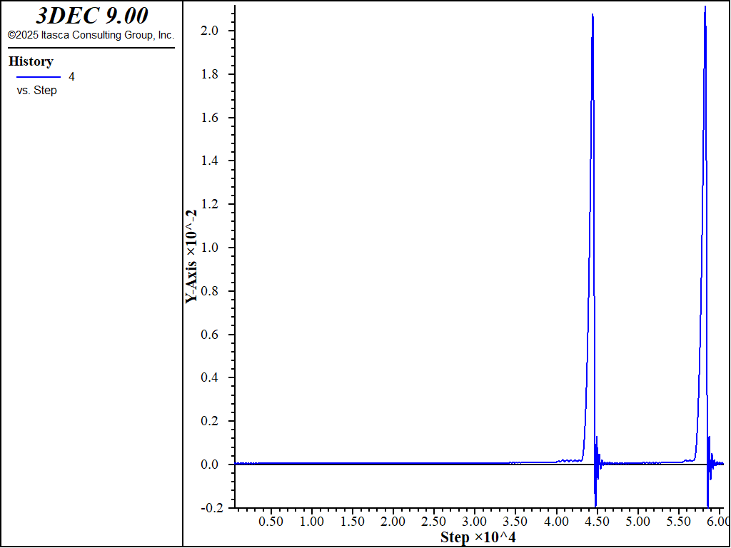
Figure 8: Shear velocity versus shear displacement in the Softening-Healing-Mohr-Coulomb joint model with \(D_c\) = 1e-4.

To test changing dilation, the test was run three more times: with a constant dilation of 10 degrees, with a constant dilation of 2 degrees, and with dilation evolving from 10 to 2 over a critical slip distance of \(D_c\) of 1e-4. Graphs of normal displacement versus shear displacement for the three cases are shown in Figure 9.

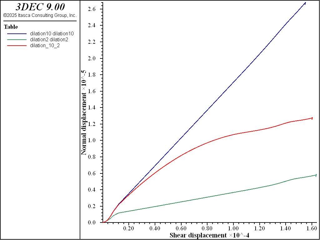
Figure 9: Normal displacement versus shear displacement for constant dilation angle of 10 degrees, constant dilation angle of 2 degrees, and a dilation angle evolving from 10 to 2 degrees.

Data Files

spring-slider.dat

model new
model random 10000
model configure energy
model large-strain off

; slider brick
block create brick -1 1 -1 1 -1 1

; spring brick
block create brick 1 3 -1 1 -1 1

; base brick
block create brick -1.5 3.5 -1.5 1.5 -1.5 -1

block zone generate edgelength 0.5

block zone cmodel assign elastic
block zone property density 2000 bulk 1e11 shear 0.6e11

; spring
block contact jmodel assign elastic
block contact property stiffness-normal 1e9 stiffness-shear 1e9

;slider-base contact - mohr-coulomb with 0 friction
block hide range position-x -1 1 position-z -1 1
block contact jmodel assign mohr
block contact property stiffness-normal 1e11 stiffness-shear 1e11
block hide off

; sliding contacts
block hide range position-x 1 3 position-z -1 1
block contact jmodel assign softening-mohr

; joint properties
block contact property stiffness-normal 1e11 stiffness-shear 1e11 ...
                   friction 25 friction-residual 20 tension 1e12 dc 1e-4

block hide off

block insitu stress 0 0 -1e6 0 0 0
block face apply stress-zz -1e6 range position-z 1
block fix range position-z -1.5 -1

model solve

model save 'blocks'

=====================================

block gridpoint initialize displacement 0 0 0
block contact reset displacement

; ==== FISH forigin histories =====
[cxi0 = block.subcontact.near(0,0,0)]
fish define sh_mu
  sh_mu = block.subcontact.prop(cxi0,'friction-current')
  sh_slip = block.subcontact.prop(cxi0,'slip')
end

block gridpoint apply velocity-x 1.0e-3 range position-x 2.9 3.1
block contact history stress-normal position 0 0 0
block contact history stress-shear position 0 0 0
block contact history displacement-shear position 0 0 0

; get velocity
block hide range position-z -1.5 -1
block history velocity-x position 0 0 0
block hide off

fish history sh_mu
fish history sh_slip

block history fob

model save 'initial'

================================

; dc = 1e-4
model restore 'initial'

history interval 100
model cycle 30000
history interval 10
model cycle 30000

model save 'spring-slider-dc1e-4'

===========================================

; dc 1e-5
model restore 'initial'
block hide range position-x 1 3 position-z -1 1
block contact property dc 1e-5
block hide off

history interval 100
model cycle 30000
history interval 10
model cycle 25000

model save 'spring-slider-dc1e-5'

========================================

dilation.dat

; File to test changing dilation angle with slip

model restore 'blocks'

block gridpoint initialize displacement 0 0 0
block contact reset displacement

block gridpoint apply velocity-x 1.0e-3 range position-x 2.9 3.1

block contact history stress-normal position 0 0 0
block contact history stress-shear position 0 0 0
block contact history displacement-shear position 0 0 0
block contact history displacement-normal position 0 0 0

; function to compute dilation
fish define get_dilation
  local cx0 = block.subcontact.near(0,0,0)
  local ndis = block.subcontact.dis.norm(cx0)
  local sdis = math.mag(block.subcontact.dis.shear(cx0))
  global dilation = math.atan(ndis/sdis)/math.degrad
  local status = io.out('Dilation = '+string(dilation))
end

model save 'initial'

; ========= dilation constant 10 =============

; set joint properties
block hide range position-x 1 3 position-z -1 1
block contact property dilation 10
block hide off

history interval 100
model cycle 30000
history interval 10
model cycle 15000

[get_dilation]

history export '4' vs '3' table 'dilation10'
table 'dilation10' export 'dilation10.tab'

; ========= dilation constant 2 =============

model restore 'initial'

; set joint properties
block hide range position-x 1 3 position-z -1 1
block contact property dilation 2
block hide off

history interval 100
model cycle 30000
history interval 10
model cycle 15000

[get_dilation]

history export '4' vs '3' table 'dilation2'
table 'dilation2' export 'dilation2.tab'

; ========= dilation changing from 10 to 2 =============

model restore 'initial'

; set joint properties
block hide range position-x 1 3 position-z -1 1
block contact property dilation 10 dilation-residual 2
block hide off

history interval 100
model cycle 30000
history interval 10
model cycle 15000

[get_dilation]

history export '4' vs '3' table 'dilation_10_2'
table 'dilation10' import 'dilation10.tab'
table 'dilation2' import 'dilation2.tab'

Properties

softening-mohr

alpha f

An exponent (>= 1) that dictates the severity of friction drop. If alpha = 0, the linear friction reduction relationship is used.

cohesion f

Joint cohesion.

cohesion-residual f

Residual joint cohesion.

dc f

Slip distance over which friction reduces from peak to residual friction.

dilation f

Joint dilation angle in degrees.

dilation-zero f

Shear displacement at which joint will cease to dilate.

friction f

Peak friction angle in degrees.

friction-current f

Current friction angle in degrees (read only).

friction-residual f

Residual joint friction angle in degrees.

healing b

If set to true, friction recovers to the peak value when slipping stops. Default is true.

slip

Plastic shear slip (read only).

stiffness-normal f

Joint normal stiffness (stress / distance).

stiffness-shear f

Joint shear stiffness (stress / distance).

tension f

Tensile strength.

tension-residual f

Residual joint tensile tensile.

References

Rice, J., 1983. “Constitutive relations for fault slip and earthquake instabilities,” Pure Appl. Geoph., 116, 790-806, 1983.