Burger’s Model

Burger’s model simulates creep mechanisms by using a Kelvin model and a Maxwell model connected in series in both the normal and shear directions.

Introduction

The Burger’s model provides a Kelvin model acting in series with a Maxwell model, in both the normal and shear directions. The Kelvin model is the combination of linear spring and dashpot components that act in parallel. The Maxwell model, on the other hand, is the combination of linear spring and dashpot components that act in series. Burger’s model acts over a vanishingly small area, and thus transmits only a force.

Behavior Summary

The rheological components of the Burger’s model are shown in Figure 1 for both the normal and shear directions. In both directions, the model combines Kelvin and Maxwell models acting in series. In the normal direction, the Kelvin model provides a linear spring with stiffness \(K_{k_n}\) and a dashpot with viscosity \(C_{k_n}\), and the Maxwell model provides a linear spring with stiffness \(K_{m_n}\) and a dashpot with viscosity \(C_{m_n}\). The Burger’s model can sustain tensile forces (\(M_t=0\)) or not (\(M_t=1\)). In the shear direction, , the Kelvin model provides a linear spring with stiffness \(K_{k_s}\) and a dashpot with viscosity \(C_{k_s}\), and the Maxwell model provides a linear spring with stiffness \(K_{m_s}\) and a dashpot with viscosity \(C_{m_s}\). A slider with friction coefficient \(f_s\) limits the value of the shear force according to a Coulomb law.

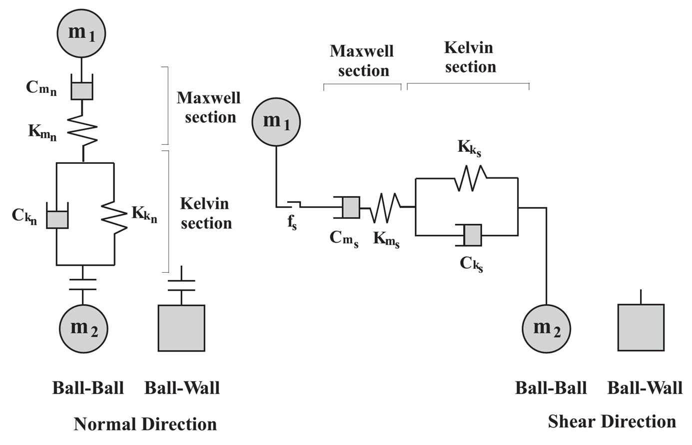
Figure 1: Rheological components of the Burger’s model.

In each direction, the total displacement of the Burger’s model, \(u\), is the sum of the displacement of the Kelvin section (\(u_k\)) and that of the Maxwell section ( \(u_{m_K}\) , \(u_{m_C}\) ) of the model:

(1)\[u = u_k + u_{m_K} + u_{m_C}\]

The first and second derivatives of the equation above are given by :

(2)\[\begin{split}\dot{u} = \dot{u}_k + \dot{u}_{m_K} + \dot{u}_{m_C} \\ \ddot{u} = \ddot{u}_k + \ddot{u}_{m_K} + \ddot{u}_{m_C}\end{split}\]

The contact forces, \(f\), using the Kelvin section and the first derivative, are given by (3). Note that symbols \(\pm\) and \(\mp\) correspond to the cases of normal and shear direction, respectively (For example, \(\pm\) means \(+\) for normal direction and \(-\) for shear direction.).

(3)\[\begin{split}f = \pm K_k u_k \pm C_k \dot{u}_{k} \\ \dot{f} = \pm K_k \dot{u}_k \pm C_k \ddot{u}_{k}\end{split}\]

Also, using stiffness \(K_m\) and viscosity of the Maxwell section:

(4)\[\begin{split}f = \pm K_m u_{m_K} \\ \dot{f} = \pm K_m \dot{u}_{m_K} \\ \ddot{f} = \pm K_m \ddot{u}_{m_K} \\ f = \pm C_m \dot{u}_{m_C} \\ \dot{f} = \pm C_m \ddot{u}_{m_C} \\\end{split}\]

Using Eqs (2) through (4), the second-order differential equation for contact force \(f\) is given by:

(5)\[f + \left[ \frac{C_k}{K_k} + C_m \left(\frac{1}{K_k}+\frac{1}{K_m}\right)\right]\dot{f} + \frac{C_k C_m}{K_k K_m} \ddot{f} = \pm C_m \dot{u} \pm \frac{C_k C_m}{K_k} \ddot{u}\]

The force at a given step can be updated based on its value at the previous step and on values of the displacements at the current step and at the previous steps, using a finite dfifference scheme described below.

Activity-Deletion Criteria

A contact with the Burger’s model is active if and only if the contact gap (\(g_{c}\)) is less than or equal to zero. The force-displacement law is skipped for inactive contacts.

Force-Displacement Law

The force-displacement law for the Burger’s model updates the contact force and moment:

(6)\[\mathbf{F_{c}} =\mathbf{F} ,\quad \mathbf{M_{c}} \equiv 0\]

where \(\mathbf{F}\) combines the contributions from the Kelvin and Maxwell models acting in series. \(\mathbf{F}\) is resolved into normal and shear forces:

(7)\[\mathbf{F} =-F_{n} {\kern 1pt} \hat{\mathbf{n}}_\mathbf{c} +\mathbf{F_{s}}\]

where \(F_{n} >0\) is tension. The shear force lies on the contact plane, and is expressed in the contact plane coordinate system:

(8)\[\mathbf{F_{s}} =F_{ss} {\kern 1pt} \hat{\mathbf{s}}_\mathbf{c} +F_{st} {\kern 1pt} \hat{\mathbf{t}}_\mathbf{c} \; \; \left({\rm 2D\; model:\; }F_{ss} \equiv 0\right).\]

From the second equation in (3) of the Kelvin section:

(9)\[\dot{u}_k = \frac{-K_k u_k \pm f}{C_k}\]

By using a central difference approximation of the finite difference scheme for the time derivative and taking average values for \(u_k\) and \(f\):

(10)\[\frac{u_k^{t+1} - u_k^{t}}{\Delta t} = \frac{1}{2 C_k} \left[-K_k \left(u_k^{t+1}+u_k^{t}\right) \pm \left( f^{t+1}+f^t \right)\right]\]

Therefore,

(11)\[u_k^{t+1} = \frac{1}{A} \left[ B u_k^t \pm \frac{\Delta t}{2 C_k}\left( f^{t+1} + f^t \right)\right]\]

where:

(12)\[\begin{split}A = 1 + \frac{K_k \Delta t}{2 C_k} \\ B = 1 - \frac{K_k \Delta t}{2 C_k}\end{split}\]

For the Maxwell section, the displacement and the first derivative are given by:

(13)\[\begin{split}u_m = u_{m_K} + u_{m_C} \\ \dot{u}_m = \dot{u}_{m_K} + \dot{u}_{m_C}\end{split}\]

Substituting the second and fourth equations of (4) into the second equation above:

(14)\[\dot{u}_m = \pm \frac{\dot{f}}{K_m} \pm \frac{f}{C_m}\]

By using a central difference approximation of the finite difference scheme and taking the average value for \(f\),

(15)\[ \frac{u_m^{t+1} - u_m^{t}}{\Delta t} = \pm \frac{f^{t+1}-f^t}{K_m \Delta t} \pm \frac{f^{t+1}+f^t}{2 C_m}\]

Therefore,

(16)\[ u_m^{t+1} = \pm \frac{f^{t+1}-f^t}{K_m} \pm \frac{\Delta t \left(f^{t+1}+f^t\right)}{2 C_m} + u_m^t\]

The total displacement and the first derivative of the Burger’s model are given by:

(17)\[\begin{split}u = u_k + u_m \\ \dot{u} = \dot{u}_k + \dot{u}_m\end{split}\]

By using the finite difference scheme for the time derivative,

(18)\[u^{t+1} - u^t = u_k^{t+1} - u_k^t + u_m^{t+1} - u_m^t\]

Substituting Eqs (11) and (16) into the equation above, the contact force, \(f^{t+1}\), is given by:

(19)\[f^{t+1} = \pm \frac{1}{C} \left[ u^{t+1} - u^t + \left(1 - \frac{B}{A}\right) u_k^t \mp D f^t \right]\]

Where:

(20)\[\begin{split}C = \frac{\Delta t}{2 C_k A} + \frac{1}{K_m} + \frac{\Delta t}{2 C_m} \\ D = \frac{\Delta t}{2 C_k A} - \frac{1}{K_m} + \frac{\Delta t}{2 C_m}\end{split}\]

The contact force \(f^{t+1}\) can be calculated from know values for \(u^{t+1}\), \(u^t\), \(u_k^t\) and \(f^t\).

The force-displacement law for the Burger’s model consists of the following steps.

1. Update the normal force \(F_{n}\) according to Eq. (19).

2. Update the shear force as follows:

   • Update the shear force \(\mathbf{F}_{s}\) according to Eq. (19).

   • Compute the shear strength:

     (21)\[F_{s}^{*} = - f_s F_{n} .\]

   • Update the linear shear force:

     (22)\[\begin{split}\mathbf{F}_{s} = \left\{\begin{array}{l} {\qquad \mathbf{F}_{s} ,\qquad \left\| \mathbf{F}_{s} \right\| \le F_{s}^{*} } \\ {\qquad F_{s}^{*} \left({\mathbf{F}_{s} \mathord{\left/ {\vphantom {\mathbf{F}_{s} \left\| F_{s}^{*} \right\| }} \right.} \left\| \mathbf{F}_{s} \right\| } \right),\qquad {\rm otherwise.}} \end{array}\right.\end{split}\]

   • Update the slip state:

     (23)\[\begin{split}s=\left\{\begin{array}{l} {\qquad {\rm true},\qquad \left\| \mathbf{F}_{s} \right\| = F_{s}^{*} } \\ {\qquad {\rm false},\qquad {\rm otherwise.}} \end{array}\right.\end{split}\]

     If the slip state is true, then the contact is sliding. Whenever the slip states changes, the slip_change callback event occurs.

Energy Partitions

The Burger’s model does not provide any energy partition.

Properties

The properties defined by the Burger’s contact model are listed in the table below as a concise reference; see the Contact Properties section for a description of the information in the table columns.

Table 1: Burger’s Model Properties

Keyword	Symbol	Description	Type	Range	Default	Modifiable	Inheritable
burger		Model name
bur_knk	\(K_{k_n}\)	Normal stiffness Kelvin section [force/length]	FLT	\([0.0,+\infty)\)	0.0	YES	NO
bur_cnk	\(C_{k_n}\)	Normal viscosity Kelvin section [force×time/length]	FLT	\([0.0,+\infty)\)	0.0	YES	NO
bur_knm	\(K_{m_n}\)	Normal stiffness Maxwell section [force/length]	FLT	\([0.0,+\infty)\)	0.0	YES	NO
bur_cnm	\(C_{m_n}\)	Normal viscosity Maxwell section [force×time/length]	FLT	\([0.0,+\infty)\)	0.0	YES	NO
bur_ksk	\(K_{k_s}\)	Shear stiffness Kelvin section [force/length]	FLT	\([0.0,+\infty)\)	0.0	YES	NO
bur_csk	\(C_{k_s}\)	Shear viscosity Kelvin section [force×time/length]	FLT	\([0.0,+\infty)\)	0.0	YES	NO
bur_ksm	\(K_{m_s}\)	Shear stiffness Maxwell section [force/length]	FLT	\([0.0,+\infty)\)	0.0	YES	NO
bur_csm	\(C_{m_s}\)	Shear viscosity Maxwell section [force×time/length]	FLT	\([0.0,+\infty)\)	0.0	YES	NO
bur_fric	\(f_s\)	Friction coefficient [-]	FLT	\([0.0,+\infty)\)	0.0	YES	NO
bur_mode	\(M_t\)	Normal-force tensile mode [-]	INT	\(\{0,1\}\)	0	YES	NO
		\(\;\;\;\;\;\;\begin{cases} \mbox{0: with tensile force} \\ \mbox{1: without tensile force} \end{cases}\)
bur_slip	\(s\)	Slip state [-]	BOOL	{false,true}	false	NO	N/A
		\(\;\;\;\;\;\;\begin{cases} \mbox{true: slipping} \\ \mbox{false: not slipping} \end{cases}\)
bur_force	\(\mathbf{F}\)	Total force (contact plane coord. system)	VEC	\(\mathbb{R}^3\)	\(\mathbf{0}\)	NO	NO
		\(\left( -F_n,F_{ss},F_{st} \right) \quad \left(\mbox{2D model: } F_{ss} \equiv 0 \right)\)

Surface Property Inheritance

The Burger’s model does not provide property inheritance capabilities.

Methods

The Burger’s model does not provide any method.

Callback Events

Table 2: Burger’s Model Callback Events

Event	Array Slot	Value Type	Range	Description
contact_activated				Contact has become active
	1	C_PNT	N/A	Contact pointer
slip_change				Slip state has changed
	1	C_PNT	N/A	Contact pointer
	2	INT	{0,1}	Slip change mode
				\(\;\;\;\;\;\;\begin{cases} \mbox{0: slip has initiated} \\ \mbox{1: slip has ended} \end{cases}\)

Usage and Verification Examples

The Verification Problem “Burger’s Contact Model: Stress Relaxation” compares the time-decay of the normal force to the expected analytical solution.

Model Summary

An alphabetical list of the linear model properties is given here.

• Burger’s Model Properties