Johnson-Kendall-Roberts (JKR) Contact Model

Introduction

Cohesion or adhesion can be modeled by introducing an attractive force component to the contact model. The terms cohesion and adhesion are usually defined for attracting forces between similar and dissimilar materials respectively. However, here the two terms are used interchangeably.

The Johnson-Kendall-Roberts (JKR) contact model is an extension of the well-known Hertz contact model proposed by [Johnson1971]. The model accounts for attraction forces due to van der Waals effects. The model is, however, also used to model material where the adhesion is caused by capillary or liquid-bridge forces ([Hærvig2017], [Carr2016], [Morrisey2013b], [Xia2019]).

The implementation of this model in PFC was first proposed as a C++ Plugin for PFC version 6.0 by Prof. Corné Coetzee, whose contribution is gratefully acknowledged. The model for PFC 6.0 was made publicly available in the UDM Library on the Itasca website.

This model is incorporated as a built-in model in PFC 7.0. It is referred to in commands and FISH by the name jkr.

Behavior Summary

The JKR contact model is an extension of the Hertz-Mindlin model, which allows for tensile forces to develop due to surface adhesion. This model also incorporates viscous damping and rolling resistance mechanisms similar to those of the Rolling Resistance Linear Model.

Activity-Deletion Criteria

A contact with the JKR model becomes active when the surface gap becomes less or equal to the reference gap. Once activated, the contact remains active until the surface gap reaches a threshold positive tear-off distance. Note that a simplified version of the model may be used where the tear-off distance is set equal to the contact reference gap.

Force-Displacement Law

The force-displacement law for the JKR model updates the contact force and moment as:

(1)\[\mathbf{F_{c}} =\mathbf{F^{JKR}} +\mathbf{F^{d}} ,\quad \mathbf{M_{c}} = \mathbf{M^r}\]

where \(\mathbf{F^{JKR}}\) is a non-linear force, \(\mathbf{F^{d}}\) is the dashpot force, and \(\mathbf{M^r}\) is the rolling resistance moment. The non-linear force (resolved into normal and shear components \(\mathbf{F^{JKR}} = F_{n}^{JKR} {\kern 1pt} \hat{\mathbf{n}}_\mathbf{c} +\mathbf{F_{s}^{JKR}}\)), the dashpot force, and the rolling resistance moment are updated as detailed below.

Normal Force \(F_{n}^{JKR}\)

Following [Johnson1971] and [Chokshi1993], an attractive force component can be introduced to the classic Hertz model, which acts over the circular contact patch area with radius \(a\),

(2)\[F_{adh} = \pi a^2 \gamma^*\]

where \(\gamma^*\) is an effective surface energy per unit area. For two dissimilar surfaces the effective surface energy is given by

(3)\[\gamma^* = \gamma_1 + \gamma_2 - 2 \gamma_{12}\]

where \(\gamma_1\) and \(\gamma_2\) are the surface energy of each surface, and \(\gamma_{12}\) is the interface energy. When the two surface materials are identical, \(\gamma_1 = \gamma_2 = \gamma\), the interface energy is zero, \(\gamma_{12} = 0\), and the effective surface energy reduces to

(4)\[\gamma^* = 2 \gamma\]

and the attractive force becomes:

(5)\[F_{adh} = 2 \pi a^2 \gamma\]

Due to the contact stress distribution the total contact normal force is given by:

(6)\[F_{n}^{JKR} = \frac{4E^* a^3}{3 \bar{R}} - \sqrt{16 \pi \gamma E^* a^3}\]

where the first term is identical to the elastic Hertz force (with \(\bar{R}\) the effective contact radius), and the second term is the adhesion component. Due to the attractive force, the contact area is larger than that predicted by the Hertz theory and the contact patch radius \(a\) is obtained by solving for the positive root of equation (6)

(7)\[a^3 = \frac{3 \bar{R}}{4E} \left[ F_{n}^{JKR} + 6 \pi \gamma \bar{R} + \sqrt{F_{n}^{JKR} 12 \pi \gamma \bar{R} + \left( 6 \pi \gamma \bar{R}\right)^2} \right]\]

The Hertz relation between the contact patch radius \(a\) and the normal deformation (\(a=\sqrt{\bar{R}\delta_n}\)) no longer holds. According to the JKR theory, the normal deformation is related to the contact radius according to the following non-linear expression,

(8)\[\delta_n = \frac{a^2}{\bar{R}} - \sqrt{\frac{4 \pi \gamma a}{E^*}}\]

In PFC the contact overlap \(\delta_n\) is readily available, and from this the contact patch radius \(a\) should be calculated. Solving equation (8) for the contact patch radius is however not trivial. [Parteli2014] proposed an analytical solution based on a fourth-order expansion of this equation and solving for the real root that is larger than the patch radius of the classic Hertz model, which yields

(9)\[\begin{split}\begin{array}{lll} & a &= \frac{1}{2} \left(w + \sqrt{w^2 - 4(c_2+s+\lambda} \right) \\ \mbox{with} & c_0 &= \bar{R}^2 \delta_n^2 \\ & c_1 &= -8(1-\nu^2)\frac{\pi\gamma\bar{R}^2}{E^*} \\ & c_2 &= -2\bar{R} \delta_n \\ & P &= -\frac{c_2^2}{12} - c_0 \\ & Q &= -\frac{c_2^3}{108} + \frac{c_0c_2}{3} - \frac{c_1^2}{8} \\ & U &= \left( - \frac{Q}{2} + \sqrt{\frac{Q^2}{4} + \frac{P^3}{27}}\right)^{1/3} \\ & s &= \left\{ \begin{array}{ll} -\frac{5c_2}{6} + U - \frac{P}{3U} & \mbox{if $P \neq 0$} \\ -\frac{5c_2}{6} - Q^{1/3} & \mbox{if $P = 0$} \end{array} \right. \\ & w &= \sqrt{c_2+2s} \\ & \lambda &= \frac{c_1}{2w} \end{array}\end{split}\]

This value of \(a\) is then used to compute \(F_{n}^{JKR}\) using equation (6).

The maximum tensile force is defined as the pull-off force \(F_{po}\) ([Chokshi1993]),

(10)\[F_{po} = 3 \pi \gamma \bar{R}\]

The pull-off force is independent on the elastic properties and only a function of particle size and surface adhesion energy. The contact force \(F_{n}^{JKR}\) can be normalized using \(F_{po}\) and plotted as a function of the normalized overlap \(\delta_n / \delta_{to}\), where the tear-off distance \(\delta_{to}\) is the separation distance at which the contact breaks under tension:

(11)\[\delta_{to} = \frac{1}{2} \frac{1}{6^{1/3}} \frac{a_0^2} {\bar{R}}\]

where \(a_0\) is the contact patch radius where \(F_{n}^{JKR}=0\), i.e., at the point where the contact is in equilibrium when no other external forces are acting:

(12)\[a_0 = \left( \frac{9\pi \gamma \bar{R}^2}{E^*} \right)^{1/3}\]

Plotting the normalized force \(F_{n}^{JKR} / F_{po}\) an normalized patch radius \(a / a_0\) against the normalized overlap \(\delta_n / \delta_{to}\) results in Figure 1 below. When two particles approach each other, the contact is formed when the two particles physically touch at \(\delta_n = 0\) (point 3 in Figure 1). At this point, the force suddenly jumps to a value \(F_{n}^{JKR} = - 8/9 F_{po}\), with the contact patch radius \(a = (2/3)^{2/3} a_0\). This attractive force will pull the particles closer until the equilibrium point is reached (assuming no other forces are acting) where \(F_{n}^{JKR} =0\), \(a = a_0\), and \(\delta_n = (4/3)^{2/3} \delta_{to}\) (point 4 in Figure 1). Further loading due to external forces will result in an increased positive overlap \(\delta_n\) and an increase in the compressive force as defined by equation (6).

Upon unloading, the same path is followed up to zero overlap \(\delta_n=0\), after which the force will further decrease down to a minimum value \(F_{n}^{JKR} = - F_{po}\) due to the necking effect where \(a = (1/2)^{2/3} a_0\) (point 2 in Figure 1). With further unloading, the force increases to a value \(F_{n}^{JKR} = - 5/9 F_{po}\) where the contact suddenly breaks (tear-off) and the force jumps to zero (point 1 in Figure 1). At this point the overlap is given by \(\delta_n = - \delta_{to}\) and the patch radius by \(a = (1/6)^{2/3} a_0\).

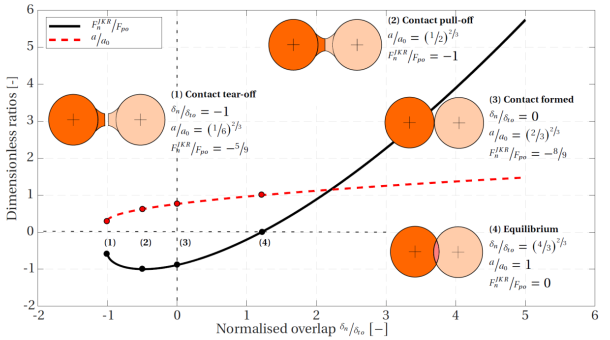
Figure 1: Normalized force and normalized contact patch radius of the JKR model as a function of the normalized overlap.

Note that the normal force is in tension when the overlap is positive \(\delta_n > 0\) and between points 3 and 4 in Figure 1. This is different from the Hertz model, where the normal force is always compressive when the overlap is positive.

Also, in the Hertz model, the normal force becomes zero for \(\delta_n \leq 0\), while in the JKR model the contact remains active with a finite contact patch until the tear-off separation distance is reached (point 1 in Figure 1).

A simplified version of the model can be used where the normal force becomes zero for \(\delta_n \leq 0\) by setting \(M_a = 0\).

Shear Force \(\mathbf{F_{s}^{JKR}}\)

In the shear direction, a trial shear force is first computed as:

(13)\[\mathbf{F_{s}^{JKR^*}} = \left(\mathbf{F_{s}^{JKR}}\right)_o + k_s^t \Delta \pmb{δ} _\mathbf{s}\]

where \(\left(\mathbf{F_{s}^{JKR}}\right)_o\) is the shear force at the beginning of the timestep, \(\Delta \pmb{δ} _\mathbf{s}\) is the relative shear-displacement increment, and the tangent shear stiffness \(k_s^t\) is given by [Marshall2009b]:

(14)\[k_s^t = 8 G^* a\]

where \(G^*\) is the effective shear modulus. The tangent shear stiffness is a function of the patch radius \(a\) and not the normal overlap as in the Hertz model, because the patch radius can be present for negative overlap until the contact breaks.

To account for cohesive effects in the tangential direction, the Coulomb friction limit is usually modified. This is a relatively simple approach that is easy to implement and is based on the work by [Thornton1991] and [ThorntonAndYin1991], who showed that, with adhesion present, the contact area decreases with an increase in the tangential force. The tangential force reaches a critical value, which defines the transition from a “peeling” action to a “sliding” action. Assuming the JKR theory ([Johnson1971a]), it is shown that at this critical point the contact area corresponds to a Hertzian-like normal stress distribution under a load of \((F_n^{JKR} + 2 F_{po})\) ([Marshall2009b]):

(15)\[\begin{split}\mathbf{F_{s}^{JKR}} = \left\{ \begin{array}{l} \mathbf{F_{s}^{JKR^*}} , {\kern 5pt} \mbox{if $\left|\mathbf{F_{s}^{JKR^*}}\right| \leq \mu (F_n^{JKR} + 2 F_{po})$} \\ \mu (F_n^{JKR} + 2 F_{po}) \left( \frac{\mathbf{F_{s}^{JKR^*}}}{\left|\mathbf{F_{s}^{JKR^*}}\right|} \right), {\kern 1pt} \mbox{otherwise} \end{array} \right.\end{split}\]

If the first condition is met, the boolean slip state is set to \(s=\mbox{false}\), and when the second condition is met it is set to \(s=\mbox{true}\). Whenever the slip states changes, the slip_change callback event occurs.

Dashpot force

The dashpot force is resolved into normal and shear components:

(16)\[\mathbf{F^{d}} =-F_{n}^{d} {\kern 1pt} \hat{\mathbf{n}}_\mathbf{c} +\mathbf{F_{s}^{d}}\]

In the normal direction:

(17)\[F_{n}^{d} = 2 \beta_n \sqrt{m_c k_n^t} \dot{\delta}_n\]

where \(m_c = \frac{m_1 m_2}{m_1 + m_2}\) is the effective contact mass with \(m_1\) and \(m_2\) the mass of the two contacting particles (for a contact with a wall facet, \(m_c = m_p\) where \(m_p\) is the mass of the particle), \(\dot{\delta}_n\) is the relative normal translational velocity, \(k_n^t\) is the tangent normal stiffness, and \(\beta_n\) is the normal critical damping ratio. This ratio takes a value \(\beta_n=0\) when there is no damping, and \(\beta_n=1\) when the system is critically damped.

The tangent normal stiffness is given by:

(18)\[k_n^t = 2 E^* a\]

The dashpot force in the shear direction is given by:

(19)\[\begin{split}\mathbf{F_s^d} = \left\{ \begin{array}{ll} \left( - 2 \beta_s \sqrt{m_c k_s^t} \right) \dot{\pmb{δ}}_\mathbf{s}, & \mbox{$s =$ false or $M_d = 0$ (full shear)} \\ \mathbf{0}, & \mbox{$s =$ true and $M_d = 1$ (slip-cut)} \end{array} \right.\end{split}\]

where \(M_d\) is the dashpot behavior mode, \(\dot{\pmb{δ}}_\mathbf{s}\) is the relative shear translational velocity, \(\beta_s\) is the shear critical damping ratio, and \(k_s^t\) is the tangential shear stiffness given by equation (14).

Rolling Resistance

The rolling resistance moment is first incremented as:

(20)\[\mathbf{M^r} :=\mathbf{M^r} - k_r^t {\kern 1pt} \Delta \pmb{θ}_\mathbf{b}\]

where \(k_r^t\) is the tangent rolling resistance stiffness, and \(\Delta \pmb{θ}_\mathbf{b}\) is the relative bend-rotation increment of Equation (12) of the “Contact Resolution” section.

The tangent rolling resistance stiffness \(k_r^t\) is defined as:

(21)\[k_r^t = k_s^t {\kern 1pt} \bar{R}^{2}\]

with \(k_s^t\) the tangent shear stiffness given by equation (14) and \(\bar{R}\) the contact effective radius(equation :eq:’cmjkr_eqR’) CS: maybe this is cmeepa_eqR??? see line 262 (the cmeepa_Mr2 equation reference) for more badness).

The magnitude of the updated rolling resistance moment is then checked against a threshold limit:

(22)\[\begin{split}\mathbf{M^r} = \left\{ \begin{array}{l} \mathbf{M^r} , {\kern 5pt} \mbox{if $\| \mathbf{M^r} \| \le \mu_r \bar{R} (F_n^{JKR} + 2 F_{po})$} \\ \mu_r \bar{R} (F_n^{JKR} + 2 F_{po}) \bigl( \frac{\mathbf{M^r}} {\| \mathbf{M^r} \|} \bigr), {\kern 1pt} \mbox{otherwise.} \end{array} \right.\end{split}\]

where the same arguments as used for the shear force are used to increase the limiting moment by the effects of the pull-off force \(F_{po}\). The normal force \(F_n^{JKR}\) is taken at the end of the current step, and \(\mu_r\) is the rolling coefficient of friction. If the first condition in (22) is met, then the rolling slip state is set to \(s_r=\mbox{false}\), and when the second condition is met it is set to \(s_r=\mbox{true}\)

Energy Partitions

The JKR model provides five energy partitions:

• strain energy, \(E_{k}\), stored in the non-linear springs;

• slip energy, \(E_{\mu}\), defined as the total energy dissipated by frictional slip;

• dashpot energy, \(E_{\beta}\), defined as the total energy dissipated by the dashpots;

• rolling strain energy, \(E_{k_r}\), stored in the rolling linear spring; and

• rolling slip energy, \(E_{\mu_r}\), defined as the total energy dissipated by rolling slip.

If energy tracking is activated, these energy partitions are updated as follows:

1. Incrementally update the strain energy:

   (23)\[\begin{split}\begin{array}{ll} E_k := E_k & + \frac{1}{2} \left(\left(F_{n}^{JKR}\right)_o + F_{n}^{JKR}\right) \Delta \delta_n \\ & + \frac{1}{2} \left(\left(\mathbf{F_{s}^{JKR}}\right)_o + \mathbf{F_{s}^{JKR}}\right) \cdot \Delta \pmb{δ}_\mathbf{s}^\mathbf{k} \\ {\rm with} & \Delta \pmb{δ} _\mathbf{s}^{k } =\Delta \pmb{δ} _\mathbf{s} -\Delta \pmb{δ} _\mathbf{s}^{\mu} = \left(\frac{\mathbf{F_{s}^{JKR}} -\left(\mathbf{F_{s}^{JKR}} \right)_{o} }{k_{s}^t } \right) \end{array}\end{split}\]

   where \(\left(F_{n}^{JKR}\right)_o\) and \(\left(\mathbf{F_{s}^{JKR}}\right)_o\) are, respectively, the JKR normal and shear forces at the beginning of the step, and the relative shear-displacement increment has been decomposed into an elastic \(\left(\Delta \pmb{δ} _\mathbf{s}^{k} \right)\) and a slip \(\left(\Delta \pmb{δ} _\mathbf{s}^{\mu } \right)\) component, with \(k_s^t\) the tangent shear stiffness at the start of the current step (equation (14)).

2. Incrementally update the slip energy:

   (24)\[E_{\mu } :=E_{\mu } - {\tfrac{1}{2}} \left(\left(\mathbf{F_{s}^{JKR}} \right)_{o} +\mathbf{F_{s}^{JKR}} \right)\cdot \Delta \pmb{δ} _\mathbf{s}^{\mu }\]

3. Incrementally update the dashpot energy:

   (25)\[E_{\beta } :=E_{\beta } - \mathbf{F^{d}} \cdot \left(\dot{\pmb{δ} }{\kern 1pt} {\kern 1pt} \Delta t\right)\]

   where \(\dot{\pmb{δ} }\) is the relative translational velocity of Equation (10) of the “Contact Resolution” section.

4. Update the rolling strain energy:

   (26)\[E_{k_r} = \frac{1}{2} \frac{\left\| \mathbf{M^{r}} \right\| ^{2} }{k_{r}}.\]

5. Incrementally update the rolling slip energy:

   (27)\[\begin{split}\begin{array}{l} {E_{\mu_r} := E_{\mu_r} - {\tfrac{1}{2}} \biggl(\left(\mathbf{M^{r}} \right)_{o} +\mathbf{M^{r}} \biggr)\cdot \Delta \pmb{θ}_\mathbf{b}^{\mu_r} } \\ {{\rm with}\qquad \Delta \pmb{θ}_\mathbf{b}^{\mu_r} = \Delta \pmb{θ}_\mathbf{b} -\Delta \pmb{θ}_\mathbf{b}^{k} =\Delta \pmb{θ}_\mathbf{b} -\left(\frac{\mathbf{M^{r}} -\left(\mathbf{M^{r}} \right)_{o} }{k_{r}^t } \right)} \end{array}\end{split}\]

   where \(\left(\mathbf{M^{r}} \right)_{o}\) is the rolling resistance moment at the beginning of the timestep, and the relative bend-rotation increment has been decomposed into an elastic \(\Delta \pmb{θ}_\mathbf{b}^{k}\) and a slip \(\Delta \pmb{θ}_\mathbf{b}^{\mu_r}\) component, with \(k_{r}^t\) the tangent rolling stiffness. The dot product of the slip component and the rolling resistance moment occurring during the timestep gives the increment of rolling slip energy.

Additional information, including the keywords by which these partitions are referred to in commands and FISH, is provided in the table below.

Table 1: JKR Model Energies

Keyword	Symbol	Description	Range	Accumulated
JKR Group:
energy‑strain‑jkr	\(E_{k}\)	strain energy	\((-\infty,+\infty)\)	YES
energy‑slip	\(E_{\mu}\)	total energy dissipated by slip	\([0.0,+\infty)\)	YES
Dashpot Group:
energy‑dashpot	\(E_{\beta}\)	total energy dissipated by dashpots	\([0.0,+\infty)\)	YES
Rolling-Resistance Group:
energy‑rrstrain	\(E_{k_r}\)	Rolling strain energy	\([0.0,+\infty)\)	NO
energy‑rrslip	\(E_{\mu_r}\)	Total energy dissipated by rolling slip	\((-\infty,0.0]\)	YES

Properties

The properties defined by the JKR contact model are listed in the table below for concise reference. See the “Contact Properties” section for a description of the information in the table columns. The mapping from the surface inheritable properties to the contact model properties is also discussed below.

Table 2: JKR Model Properties

Keyword	Symbol	Description	Type	Range	Default	Modifiable	Inheritable
jkr		Model name
JKR Group:
jkr_shear	\(G\)	Shear modulus [stress]	FLT	\((0.0,+\infty)\)	0.0	YES	YES
jkr_poiss	\(\nu\)	Poisson’s ratio [-]	FLT	\([0.0,0.5]\)	0.0	YES	YES
ks_fac	\(k_{sf}\)	Shear stiffness scaling factor [-]	FLT	\((0.0,+\infty)\)	1.0	YES	NO
fric	\(\mu\)	Sliding friction coefficient [-]	FLT	\([0.0,+\infty)\)	0.0	YES	YES
surf_adh	\(\gamma\)	Surface adhesion energy [energy/area]	FLT	\([0.0,+\infty)\)	0.0	YES	NO
a0	\(a_0\)	Equilibrium contact patch radius [length]	FLT	\([0.0,+\infty)\)	0.0	NO	N/A
pull_off_f	\(F_{po}\)	Pull-off force [force]	FLT	\((-\infty,0.0]\)	0.0	NO	NO
tear_off_d	\(\delta_{to}\)	Tear-off distance [-]	FLT	\((0.0,1.0)\)	0.5	YES	NO
active_mode	\(M_a\)	Active mode [-]	INT	{0;1}	0	YES	NO
		\(\;\;\;\;\;\;\begin{cases} \mbox{0: no negative overlap} \\ \mbox{1: allows negative overlap} \end{cases}\)
jkr_slip	\(s\)	Slip state [-]	BOOL	{false,true}	false	NO	N/A
jkr_force	\(\mathbf{F^{JKR}}\)	JKR force (contact plane coord. system)	VEC	\(\mathbb{R}^3\)	\(\mathbf{0}\)	YES	NO
		\(\left( -F_n^{JKR},F_{ss}^{JKR},F_{st}^{JKR} \right) \quad \left(\mbox{2D model: } F_{ss}^{JKR} \equiv 0 \right)\)
Rolling-Resistance Group:
rr_fric	\(\mu_r\)	Rolling friction coefficient [-]	FLT	\([0.0,+\infty\)	0.0	YES	YES
rr_moment	\(M^r\)	Rolling Resistance moment (contact plane coord. system)	VEC	\(\mathbb{R}^3\)	\(\mathbf{0}\)	YES	NO
		\(\left( 0,M_{bs}^r,M_{bt}^r \right) \quad \left(\mbox{2D model: } M_{bt}^r \equiv 0 \right)\)
rr_slip	\(s_r\)	Rolling slip state [-]	BOOL	{false,true}	false	NO	N/A
Dashpot Group:
dp_nratio	\(\beta_n\)	Normal critical damping ratio [-]	FLT	\([0.0,1.0]\)	0.0	YES	NO
dp_sratio	\(\beta_s\)	Shear critical damping ratio [-]	FLT	\([0.0,1.0]\)	0.0	YES	NO
dp_mode	\(M_d\)	Dashpot mode [-]	INT	{0;1}	0	YES	NO
		\(\;\;\;\;\;\;\begin{cases} \mbox{0: no cutt-off} \\ \mbox{1: cut-off in shear when sliding} \end{cases}\)
dp_force	\(\mathbf{F^{d}}\)	Dashpot force (contact plane coord. system)	VEC	\(\mathbb{R}^3\)	\(\mathbf{0}\)	NO	N/A
		\(\left( -F_n^d,F_{ss}^d,F_{st}^d \right) \quad \left(\mbox{2D model: } F_{ss}^d \equiv 0 \right)\)

Surface Property Inheritance

The shear modulus \(G\), Poisson’s ratio \(\nu\), friction coefficient \(\mu\), and rolling friction coefficient \(\mu_r\) may be inherited from the contacting pieces. Remember that for a property to be inherited, the inheritance flag for that property must be set to true (default), and both contacting pieces must hold a property with the exact same name.

The shear modulus and Poisson’s ratio are inherited as:

(28)\[\begin{split}\nu &= \frac{4 G^* - E^*}{2 G^* - E^*} \\ G &= 2 G^* (2 - \nu)\end{split}\]

with:

(29)\[\begin{split}E^* &= \left( \frac{1-\nu^{(1)}}{2G^{(1)}} + \frac{1-\nu^{(2)}}{2G^{(2)}} \right)^{-1} \\ G^* &= \left( \frac{2-\nu^{(1)}}{G^{(1)}} + \frac{2-\nu^{(2)}}{G^{(2)}} \right)^{-1}\end{split}\]

where (1) and (2) denote the properties of piece 1 and 2, respectively.

The friction and rolling friction coefficients are inherited using the minimum of the values set for the pieces:

(30)\[\begin{split}\mu &= \min \left( \mu^{(1)} ,\mu^{(2)} \right) \\ \mu_r &= \min \left( \mu_r^{(1)},\mu_r^{(2)}\right)\end{split}\]

Methods

No methods are defined by the JKR model.

Callback Events

Table 3: JKR Model Callback Events

Event	Array Slot	Value Type	Range	Description
contact_activated				contact becomes active
	1	C_PNT	N/A	contact pointer
slip_change				Slip state has changed
	1	C_PNT	N/A	contact pointer
	2	INT	{0;1}	slip change mode
				\(\;\;\;\;\;\;\begin{cases} \mbox{0: slip has initiated} \\ \mbox{1: slip has ended} \end{cases}\)

Model Summary

An alphabetical list of the JKR model properties is given here.

• JKR Model Properties

References

[Carr2016]

Carr, M. J., W. Chen, K. Williams, and A. Katterfeld. “Comparative investigation on modelling wet and sticky material behaviours with a simplified JKR cohesion model and liquid bridging cohesion model in DEM,” ICBMH 2016 - 12th International Conference on Bulk Materials Storage, Handling and Transportation, Proceedings, pages 40–49, 2016.

[Chokshi1993] (1,2)

Chokshi, A.G., Tielens, G. M., and D. Hollenbach. “Dust Coagulation,” The Astrophysical Journal, 407:806-819, Apr. 1993.

[Hærvig2017]

Hærvig, J. , U. Kleinhans, C.Wieland, H. Spliethoff, A. L. Jensen, K. Sørensen, and T. J. Condra. “On the adhesive JKR contact and rolling models for reduced particle stiffness discrete element simulations,” Powder Technology, 319:472–482, 2017. ISSN 1873328X. doi:10.1016/j.powtec.2017.07.006. URL http://dx.doi.org/10.1016/j.powtec.2017.07.006.

[Johnson1971] (1,2)

Johnson, K. L., K. Kendall, and A. D. Roberts. “Surface Energy and the Contact of Elastic Solids,” Proceedings of the Royal Society of London. Series A, Mathematical and Physical Sciences, 324(1558):301–313, Sept. 1971.

[Marshall2009b] (1,2)

Marshall, J. S., “Discrete-Element Modeling of Particulate Aerosol Flows,” Journal of Computational Physics, 228(5):1541-1561, Mar. 2009, doi:10.1016/j.jcp.2008.10.035.

[Morrisey2013b]

Morrissey, J. P. “Discrete Element Modelling of Iron Ore Pellets to Include the Effects of Moisture and Fines,” PhD thesis, Edinburgh, Scotland: University of Edinburgh (2013).

[Parteli2014]

Parteli, E. J., Schmidt, J., Blümel, C., Wirth, K. E., Peukert, W., and T. Pöshel. “Attractive particle interaction forces and packing density of fine glass powders,” Scientific Reports, 4:1-7,2014. ISSN 20454322. doi:10.1038/srep06227.

[Xia2019]

Xia, R., B. Li, X.Wang, T. Li, and Z. Yang. “Measurement and calibration of the discrete element parameters of wet bulk coal,” Measurement: Journal of the International Measurement Confederation, 142:84–95, 2019. ISSN 02632241. doi: 10.1016/j.measurement.2019.04.069.