FLAC3D Theory and Background • Constitutive Models

Modified Cam-Clay Model

The modified Cam-Clay model is an incremental hardening/softening elastoplastic model. Its features include a particular form of nonlinear elasticity and a hardening/softening behavior governed by volumetric plastic strain (“density” driven). The failure envelopes are self-similar in shape and correspond to ellipsoids of rotation about the mean stress axis in the principal stress space. The shear flow rule is associated; no resistance to tensile mean stress is offered in this model. See Roscoe and Burland (1968) and Wood (1990) for detailed discussions on the modified Cam-Clay model. For convenience, we drop the qualifier “modified” in the following discussion. Also, recall that all models are expressed in terms of effective stresses. In particular, all pressures referred to in this section are effective pressures.

Formulations

Incremental Elastic Law

The generalized stress components involved in the model definition are the mean effective pressure, \(p\), and deviatoric stress, \(q\), defined as

(1)\[\begin{split}\begin{matrix} p = - {1 \over 3} \sigma_{ii} \\ \\ q = \sqrt{3J_2} \end{matrix}\end{split}\]

where the Einstein summation convention applies, and \(J_2\) is the second invariant of the effective deviatoric-stress tensor \([s]\):

(2)\[ J_2 = {{1}\over{2}} s_{ij} s_{ij}\]

The incremental strain variables associated with \(p\) and \(q\) are the volumetric strain increment, \(\Delta \epsilon_p\), and shear strain increment, \(\Delta \epsilon_q\), and we have

(3)\[\begin{split}\begin{matrix} \Delta \epsilon_p = - \Delta \epsilon_{ii} \\ \\ \Delta \epsilon_q = {2 \over 3} \sqrt{3 \Delta J_2'} \end{matrix}\end{split}\]

where \(\Delta J_2'\) stands for the second invariant of the incremental deviatoric-strain tensor \(\Delta [e]\):

(4)\[ \Delta J_2' = {{1}\over{2}} \Delta e_{ij} \Delta e_{ij}\]

In the plastic flow formulation, it is assumed that both plastic and elastic principal strain-increment vectors are coaxial with the current principal stress vector. The generalized strain increments are then decomposed into elastic and plastic parts so that

(5)\[\begin{split}\begin{matrix} \Delta \epsilon_p = \Delta \epsilon_p^e + \Delta \epsilon_p^p \\ \\ \Delta \epsilon_q = \Delta \epsilon_q^e + \Delta \epsilon_q^p \end{matrix}\end{split}\]

The evolution parameter is the specific volume, \(v\), defined as

(6)\[ v = {V \over V_s}\]

where \(V_s\) is the volume of solid particles, assumed incompressible, contained in a volume, \(V\), of soil. The incremental relation between volumetric strain, \(\epsilon_p\), and specific volume has the form

(7)\[ \Delta \epsilon_p = - {\Delta v \over v}\]

And the new specific volume, \(v^N\), for the step may be calculated as

(8)\[ v^N = v (1 - \Delta \epsilon_p)\]

The incremental expression of Hooke’s law in terms of generalized stress and strains is

(9)\[\begin{split}\begin{matrix} \Delta p = K \Delta \epsilon_p^e \\ \\ \Delta q = 3 G \Delta \epsilon_q^e \end{matrix}\end{split}\]

where \(\Delta q = \sqrt{3 \Delta J_2}\), and \(\Delta J_2\) stands for the second invariant of the incremental deviatoric-stress tensor:

(10)\[ \Delta J_2 = {{1}\over{2}} \Delta s_{ij} \Delta s_{ij}\]

In the Cam-Clay model, the tangential bulk modulus, \(K\), in the volumetric relation (Equation (9)) is updated to reflect a nonlinear law derived experimentally from isotropic compression tests. The results of a typical isotropic compression test are presented in the semi-logarithmic plot of Figure 1.

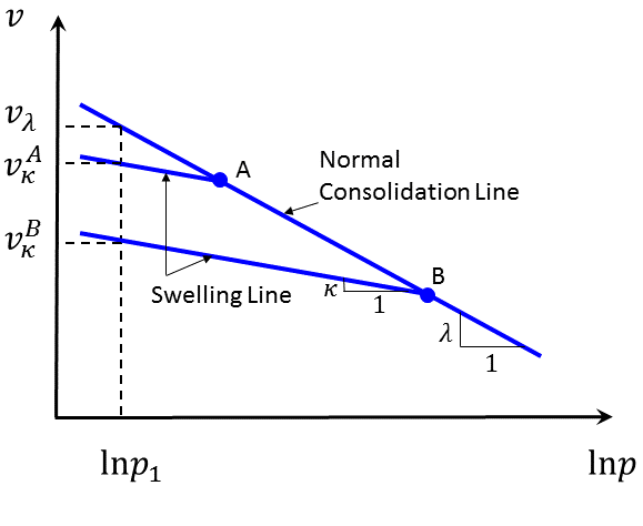
Figure 1: Normal consolidation line and unloading-reloading (swelling) line for an isotropic compression test.

As the normal consolidation pressure, \(p\), increases, the specific volume, \(v\), of the material decreases. The point representing the state of the material moves along the normal consolidation line, defined by the equation

(11)\[ v = v_{\lambda} - \lambda \ln {p \over p_1}\]

where \(\lambda\) is defined as the slope of the normal consolidation line (not to be confused with the plastic volumetric multiplier, \({\lambda}^v\), used in the plasticity flow rule given in the section on plastic correction), and \(v_{\lambda}\) are two material parameters, and \(p_1\) is a reference pressure. Note that \(v_{\lambda}\) is the value of the specific volume at the reference pressure \(p_1\). A typical value is \(p_1 = 1\) kPa.

An unloading-reloading excursion, from point \(A\) or \(B\) on the figure, will move the point along an elastic swelling line of slope \(\kappa\), back to the normal consolidation line where the path will resume. The equation of the swelling lines has the form

(12)\[ v = v_{\kappa} - \kappa \ln {p \over p_1}\]

where \(\kappa\) is a material constant, and the value of \(v_{\kappa}\) for a particular line depends on the location of the point on the normal consolidation line from which unloading was performed (i.e., \(v_{\kappa}^A\) for unloading from point \(A\), and \(v_{\kappa}^B\) for unloading from point \(B\) in Figure 1).

The recoverable change in specific volume, \(\Delta v^e\), may be expressed in incremental form after differentiation of Equation (12):

(13)\[ \Delta v^e = - \kappa {\Delta p \over p}\]

After division of both members by \(v\), and using Equation (7):

(14)\[ \Delta p = {v p \over \kappa} \Delta \epsilon_p^e\]

In the Cam-Clay model, it is assumed that any change in mean pressure is accompanied by elastic change in volume according to the preceding expression. Comparison with Equation (9), therefore, suggests the following expression for the tangent bulk modulus of the Cam-Clay material:

(15)\[ K = {v p \over \kappa}\]

Under more general loading conditions, the state of a particular point in the medium might be represented by a point, such as \(A\), located below the normal consolidation line in the \((v,\ln p)\) plane (see Figure 2). By virtue of the law adopted in Equation (12), an elastic path from that point proceeds along the swelling line through \(A\).

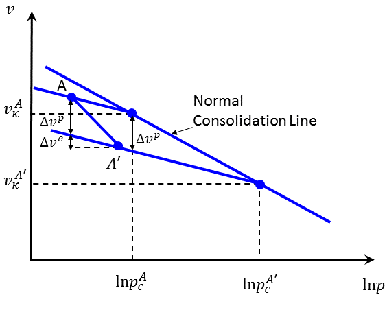
Figure 2: Plastic volume change corresponding to an incremental consolidation pressure change.

The specific volume and mean pressure at the intersection of the swelling line and normal consolidation line are referred to as (normal) consolidation (specific) volume and (normal) consolidation pressure (\(v_c^A\) and \(p_c^A\), in the case of point \(A\)). Consider an incremental change in stress bringing the point from state \(A\) to state \(A'\). At \(A'\), there is a corresponding consolidation volume, \(v_c^{A'}\), and consolidation pressure, \(p_c^{A'}\). The increment of plastic volume change, \(\Delta v^p\), is measured on the figure by the vertical distance between swelling lines (associated with points \(A\) and \(A'\)), and we can write, using incremental notation,

(16)\[ \Delta v^p = -(\lambda - \kappa) {\Delta p_c \over p_c}\]

After division of the left and right member by \(v\), we obtain, comparing with Equation (7),

(17)\[ \Delta \epsilon_p^p = {\lambda - \kappa \over v} {\Delta p_c \over p_c}\]

Hence, whereas elastic volume changes take place whenever the mean pressure changes, plastic volume changes occur only when the consolidation pressure changes.

Yield and Potential Functions

The yield function corresponding to a particular value, \(p_c\), of the consolidation pressure has the form

(18)\[ f(q,p) = q^2 + M^2 p (p - p_c)\]

where \(M\) is a material constant. The yield condition \(f\) = 0 is represented by an ellipse with horizontal axis \(p_c\) and vertical axis \(Mp_c\) in the \((q,p)\)-plane (see Figure 3). Note that the ellipse passes through the origin; hence, the material in this model is not able to support an all-around tensile stress.

The failure criterion is represented in the principal stress space by an ellipsoid of rotation about the mean stress axis (any section through the yield surface at constant mean effective stress, \(p\), is a circle).

The potential function \(g\) corresponds to an associated flow rule, and we have

(19)\[ g(p,q) = f(q,p) = q^2 + M^2 p (p - p_c)\]

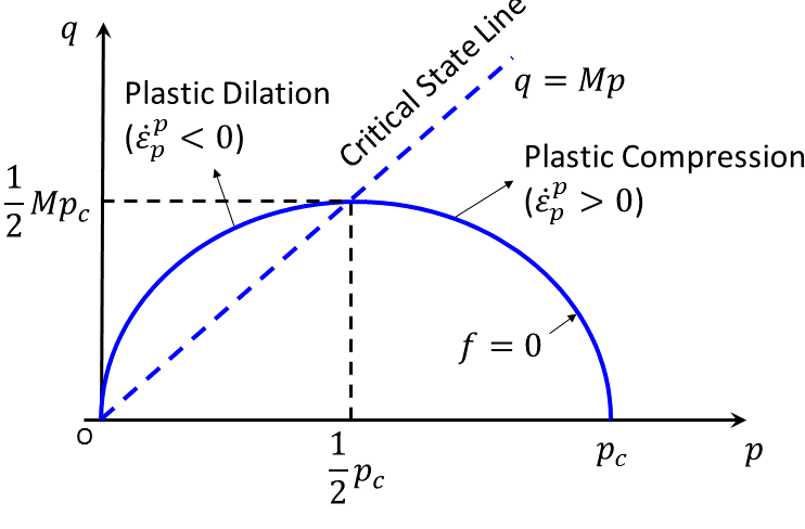
Figure 3: Cam-Clay failure criterion in FLAC3D.

Plastic Corrections

The flow rule used to describe plastic flow has the form

(20)\[\begin{split}\begin{matrix} \Delta \epsilon_p^p = \lambda^v {\partial g \over \partial p} \\ \\ \Delta \epsilon_q^p = \lambda^v {\partial g \over \partial q} \end{matrix}\end{split}\]

where \(\lambda^v\) is the plastic (volumetric) multiplier whose magnitude remains to be defined.

Using Equation (19) for \(g\), these expressions give, after partial differentiation:

(21)\[\begin{split}\begin{matrix} \Delta \epsilon_p^p = \lambda^v c_a \\ \\ \Delta \epsilon_q^p = \lambda^v c_b \end{matrix}\end{split}\]

where

(22)\[\begin{split}\begin{matrix} c_a = M^2 (2p - p_c) \\ \\ c_b = 2 q \end{matrix}\end{split}\]

The elastic strain increments may be expressed from Equation (3) as total minus plastic increments. In further using Equation (21), the elastic laws in Equation (19) become

(23)\[\begin{split}\begin{matrix} \Delta p = K (\Delta \epsilon_p - \lambda^v c_a) \\ \\ \Delta q = 3G (\Delta \epsilon_q - \lambda^v c_b) \end{matrix}\end{split}\]

Let the new and old stress states be referred to by the superscripts \(N\) and \(O\), respectively. Then, by definition, for one step:

(24)\[\begin{split}\begin{matrix} p^N = p^O + \Delta p \\ \\ q^N = q^O + \Delta q \end{matrix}\end{split}\]

Substitution of Equation (23) gives

(25)\[\begin{split}\begin{matrix} p^N = p^I - \lambda^v K c_a \\ \\ q^N = q^I - \lambda^v 3 G c_b \end{matrix}\end{split}\]

where the superscript \(I\) is used to represent the elastic guess obtained by adding to the old stresses; elastic increments are computed using the total strain increments:

(26)\[\begin{split}\begin{matrix} p^I = p^O + K \Delta \epsilon_p \\ \\ q^I = q^O + 3G \Delta \epsilon_q \end{matrix}\end{split}\]

The parameter \(\lambda^v\) may now be defined by requiring that the new stress point be located on the yield surface. Substitution of \(p^N\) and \(q^N\) (as given by Equation (25)) for \(p\) and \(q\) in \(f(q,p)\) = 0 gives, after some manipulation (see Equation (18)),

(27)\[ a (\lambda^v)^2 + b \lambda^v + c = 0\]

where

(28)\[\begin{split}\begin{matrix} a = (M K c_a)^2 + (3G c_b)^2 \\ \\ b = - \left [ K c_a c_a^I + 3G c_b c_b^I \right ] \\ \\ c = f(q^I,p^I) \end{matrix}\end{split}\]

Of the two roots of this equation, the one with the smallest magnitude must be retained.

Note that at the critical point corresponding to \(p_{cr} = p_c/2\), \(q_{cr} = M p_c/2\) in Figure 3, the normal to the yield curve \(f\) = 0 is parallel to the \(q\)-axis. Since the flow rule is associated, the plastic volumetric strain-rate component vanishes there. As a result of the hardening rule (Equation (17)), the consolidation pressure, \(p_c\), will not change. The corresponding material point has reached the critical state in which unlimited shear strains occur with no accompanying change in specific volume or stress level.

The new stress components, \(\sigma_{ij}^N\), are expressed in terms of old and new generalized stress values, using the expressions

(29)\[ {{\sigma}_{ij}}^N = {s_{ij}}^N + p^N\ {\delta}_{ij}\]

where

(30)\[ {s_{ij}}^N = {s_{ij}}^I\ \ {{q^N}\over{q^I}}\]

and \([s]\) is the deviatoric stress tensor.

Hardening/Softening Rule

The size of the yield curve is dependent on the value of the consolidation pressure, \(p_c\) (see Equation (18)). This pressure is a function of the plastic volume change, and varies with the specific volume as indicated in Equation (17). The consolidation pressure is updated for the step, using the formula

(31)\[ p_c^N = p_c (1 + \Delta \epsilon_p^p {{v}\over{\lambda - \kappa}})\]

where \(\Delta \epsilon_p^p\) is the plastic volumetric strain increment for the step, \(v\) is the current specific volume, and \(\lambda\) and \(\kappa\) are material parameters, as given previously in Equation (11).

Initial Stress State

The Cam-Clay model in FLAC3D or 3DEC is only applicable to material in which the stress state corresponds to a compressive mean effective stress. This model is not designed to predict the behavior of material in which this condition is not met. In particular, the initial state of the material (just before application of the Cam-Clay model) must be consistent with this requirement. The initial stress state may be specified using the zone initialize command, or may be the result of a run in which another constitutive model has been used. An error message will be issued if the Cam-Clay model is applied to a zone where the initial effective pressure, defined as \(p_0\), is negative.

Over-consolidation Ratio

The over-consolidation ratio, \(R\), is defined as the ratio between the zone initial pre-consolidation pressure (a material property) and initial pressure, \(p_0\):

(32)\[ R = {p_{c0} \over p_0}\]

This ratio is useful in characterizing the behavior of Cam-Clay material.

Implementation Procedure

In the implementation of the Cam-Clay model in FLAC3D/3DEC, an elastic guess, \(\sigma_{ij}^I\), is first computed after adding to the old stress components, increments calculated by application of Hooke’s law to the total strain increment for the step.

Elastic guesses for the mean pressure, \(p^I\), and deviatoric stress, \(q^I\), are calculated using Equation (1). If these stresses violate the criterion for yield and \(f(q^I,p^I) >\) 0 (see Equation (18)), plastic deformation takes place and the consolidation pressure must be updated. In this situation, a correction must be applied to the elastic guess to give the new stress state. New stresses \(p^N\) and \(q^N\) are first evaluated from Equation (25) using the expression for \(\lambda\) corresponding to the root of Equation (27) and (28) with smallest magnitude. Note that in this version of the code, the expressions in Equation (22) for \(c_a\) and \(c_b\) are evaluated using the elastic guess; the error associated with this technique is expected to be small, provided the steps are small. New stress tensor components in the system of reference axes are hence evaluated using Equation (29) and (30).

Volumetric strain increment, \(\Delta \epsilon_p\), and mean pressure, \(p\), for the zone are computed as average over all involved tetrahedra (see Equation (1) and (3)). The zone volumetric strain, \(\epsilon_p\), is incremented, and the zone specific volume, \(v\), is updated, using Equation (8). In turn, the new zone consolidation pressure is calculated from Equation (31), and the tangential bulk modulus is updated using formula (Equation (15)).

If a nonzero value for the Poisson’s ratio property is imposed, a new shear modulus is calculated from the expression \(G = 1.5(1-2 \nu) K / (1+\nu)\). Otherwise, \(G\) is left unchanged as long as the condition \(0 \leq \nu \leq\) 0.5 is satisfied; if it is not, \(G\) is assigned a value of \(\nu\) = 0 or \(\nu\) = 0.5, as appropriate.

The new values for the consolidation pressure and shear and bulk moduli are then stored for use in the next timestep. The material properties thus lag one timestep behind the corresponding calculation. In an explicit code, this error is small because the steps are small.

Determination of the Input Parameters

Frictional constant M — \(M\) is the ratio of \(q/p_{cr}\) at the critical state line. Therefore, a series of triaxial tests (drained or undrained with pore-pressure measurement) can be used to obtain this constant. These tests should be carried out to large strains to ensure that the final values of \(p_{cr}\) and \(q\) are close to the critical state line. The slope of a best-fitting line of \(q\) vs \(p_{cr}\) will be the parameter \(M\).

\(M\) is related to the effective stress friction angle, \(\phi'\), of the Mohr-Coulomb yield function. However, since the Cam-Clay critical state line is dependent on the intermediate stress \(\sigma_2\), while Mohr-Coulomb is not, the relation between \(M\) and \(\phi'\) will be different for different values of \(\sigma_2\) at yield. (This condition is similar to the relation between Mohr-Coulomb and Drucker-Prager yield functions.) For triaxial compression tests,

(33)\[ M = {{6 \sin \phi'}\over {3 - \sin \phi'}}\]

while, for triaxial extension tests,

(34)\[ M = {{6 \sin \phi'}\over {3 + \sin \phi'}}\]

The slopes of the normal consolidation and swelling lines ( \(\lambda\) and \(\kappa\)) — Ideally, these two parameters should be obtained from an isotropically loaded triaxial test (\(q\) = 0), with several unloading excursions. The slope of the normal compression line in a \(v\) versus \(\ln p\) plot will be the parameter \(\lambda\). The slope of an unloading excursion in the same plot will be the parameter \(\kappa\).

These two parameters can also be derived from an oedometer test, making certain assumptions. Let \(\sigma_v\) and \(\sigma_H\) be the vertical and horizontal stresses in an oedometer test. In most oedometer apparatus it is not possible to measure the horizontal stresses, \(\sigma_H\), so the mean stress, \(p = (\sigma_v + 2\sigma_H)/3\), is not known. However, experimental data show that the ratio of horizontal to vertical effective stresses, \(K_0\), is constant during normal compression. Since \(p = \sigma_v (1 + 2K_0)/3\) along the normal compression line, the slope of \(v\) vs \(\ln p\) will be equal to the slope of \(e\) versus \(\ln \sigma_v\), where the void ratio \(e = v - 1\).

The compression index, \(C_c\), is calculated as the slope of \(e\) vs \(\log_{10} (\sigma_v)\). So the parameter \(\lambda\) will be

(35)\[ \lambda = C_c / \ln (10) = C_c / 2.3\]

Experimental data show that along a swelling line in an oedometer test, \(K_0\) is not constant, so an estimate of \(\kappa\) based on the swelling coefficient, \(C_s\), will only be an approximation.

(36)\[ \kappa \approx C_s / \ln (10) = C_s / 2.3\]

In practice, \(\kappa\) is usually chosen in the range of 1/5 to 1/3 of \(\lambda\).

Location of the normal consolidation line in the \(v\) versus \(\ln p\) plot — In order to determine the location of the normal consolidation line in the \(v\) versus \(\ln p\) plot, a point \((v_{\lambda}\), \(\ln p_1)\) on this line must be specified. The obvious way to determine this point is to perform an isotropic triaxial test. There is an alternative way to determine this point based on the undrained shear strength (for details, see Britto and Gunn 1987).

The equation of the normal consolidation line is \(v = v_{\lambda} - \lambda \ln {{p}/{p_1}}\) (also, see Equation (11)).

The specific volume intercept, \(\Gamma\), at the critical state line for \(p = p_1\), is given (Wood 1990) by

(37)\[ \Gamma = v_{\lambda} - (\lambda - \kappa) \ln (2)\]

In a soil, the undrained shear strength, \(c_u\), is uniquely related to the specific volume, \(v_{cr}\), by the equation

(38)\[ c_u = {{M p_1} \over {2}} \exp \left({{\Gamma - v_{cr}} \over {\lambda}}\right)\]

Thus, the value of \(\Gamma\) for a given \(p_1\), and therefore \(v_{\lambda}\), can be calculated if the undrained shear strength for a particular specific volume, \(v_{cr}\), along with the parameters \(M\), \(\lambda\), and \(\kappa\), is known.

Pre-consolidation pressure, \(p_{c0}\) — The pre-consolidation pressure determines the initial size of the yield surface in the equation

(39)\[ q^2 = M^2 [p (p_{c0} - p)]\]

If a sample has been submitted to an isotropic loading path, \(p_{c0}\) will be the maximum past mean effective stress. If the sample has followed other non-isotropic paths, \(p_{c0}\) has to be calculated from the previous maximum \(p\) and \(q\), using Equation (39).

The maximum vertical effective stress can be calculated from an oedometer test using Casagrande’s method (for details, see Britto and Gunn 1987). Some hypothesis has to be made about the maximum horizontal effective stress. A common hypothesis is Jaky’s relation:

(40)\[ K_{nc} = {{\sigma_{h\max}} \over {\sigma_{v\max}}} \simeq 1 - \sin \phi'\]

where \(K_{nc}\) is the coefficient of horizontal \((\sigma_{h\max})\) to vertical \(\sigma_{v\max}\) stress at rest for normally consolidated soil. For example, if a soil with an effective friction angle of 20° has experienced a maximum vertical effective stress, \(\sigma_{v\max}\) = 1 MPa. Then, using Jaky’s relation,

\[K_{nc} = 1 - \sin 20^{\circ} = 0.658\]

and the maximum horizontal stress is

(41)\[ {\sigma_{h\max}} = 0.658 \ \hbox{MPa}\]

The maximum values of \(p\) and \(q\) are

\[p_{\max} = {{\sigma_{v\max} + 2 \sigma_{h\max}} \over {3}} = 0.772 \ {\hbox {MPa}}\]

\[q_{\max} = \sigma_{v\max} - \sigma_{h\max} = 0.342 \ {\hbox {MPa}}\]

Substituting these two values in the yield function (Equation (18)), we obtain the pre-consolidation pressure,

\[p_{c0} = p_{\max} + {{q^2_{\max}} \over {M^2 \times p_{\max}}} = 1.026 \ \hbox{MPa}\]

Initial values for specific volume, \(v_{0}\), and bulk modulus, \(K\) — Given an initial effective pressure \(p_0\), the initial specific volume \(v_0\) must be consistent with the choice of parameters \(\kappa, \lambda, p_1\), and \(p_{c0}\). The initial value \(v_0\) is calculated to correspond to the value of the specific volume corresponding to \(p_0\) on the swelling line through the point on the normal consolidation line at which \(p = p_{c0}\). From Figure 4, it follows that

(42)\[ v_0 = v_{\lambda} - \lambda \ln \left({{p_{c0}} \over {p_1}}\right) + \kappa \ln \left({{p_{c0}} \over {p}} \right)\]

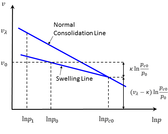
Figure 4: Determination of initial specific volume.

The initial value of the bulk modulus, \(K\), may in turn be evaluated using Equation (15), which gives

(43)\[ K_0 = {{v_0 p_0} \over {\kappa}}\]

In FLAC3D/3DEC, the default values for the properties \(v_{0}\) and \(K\) are evaluated using Equations (42) and (43). when the first step command is issued.

Note that the mean effective pressure, \(p\), must be initialized corresponding to the initial stress state before stepping begins with the Cam-Clay model. This can be done with a FISH function (e.g., in the isotropic consolidation example).

Maximum value of the elastic parameters \(K\) and \(G\) — In the Cam-Clay model, the value of the bulk modulus, \(K\), changes as a function of the specific volume and the mean stress:

(44)\[ K = {{v p} \over {\kappa}}\]

The input values of \(K_{max}\) and \(G\) are used in the mass scaling calculation performed in FLAC3D/3DEC to ensure numerical stability. This calculation is done once every time a model step command is issued. These input values should be chosen to give an upper bound to the sum \((K + 4/3 G)\), as evaluated by the model between two consecutive model step commands. Values should not, however, be set too high or the model may be slow to converge. They should be selected based on the stress level in the problem.

\(G\) or \(\nu\) — The modified Cam-Clay model in FLAC3D/3DEC allows the user to specify either a constant shear modulus or a constant Poisson’s ratio.

If no Poisson’s ratio is specified, a constant shear modulus equal to the input value is assumed. Then the Poisson’s ratio will vary as a function of the specific volume and the mean stress:

(45)\[ \nu = {{3 \left({{v p} \over {\kappa}}\right) - 2G} \over {6 \left({{v p} \over {\kappa}}\right) + 2G}}\]

If a nonzero Poisson’s ratio is specified, the shear modulus will vary at the same rate as the bulk modulus in order to maintain a constant Poisson’s ratio:

(46)\[ G = {{3 \left({{v p} \over {\kappa}}\right) (1 - 2\nu)} \over {2 \ (1 - 2\nu)}}\]

The comparison between the double-yield model and modified Cam-clay model are summarized here.

References

Wood, D.M. Soil Behaviour and Critical State Soil Mechanics. Cambridge: Cambridge University Press (1990).

Roscoe K.H., and J. B. Burland. “On the Generalised Stress-Strain Behavior of ‘Wet Clay’,” in Engineering Plasticity, pp. 535-609. J. Heyman and F. A. Leckie, eds. Cambridge: Cambridge University Press (1968).

modified-cam-clay Model Properties

Use the following keywords with the zone property (FLAC3D) or block zone property (3DEC) command to set these properties of the modified Cam-Clay model.

modified-cam-clay

bulk-maximum f

maximum elastic bulk modulus, \(K_{max}\)

kappa f

slope of elastic swelling line, \(\kappa\)

lambda f

slope of normal consolidation line, \(\lambda\)

poisson f

Poisson’s ratio, \(\nu\)

pressure-reference f

reference pressure, \(p_1\)

pressure-effective f

mean effective stress, \(p\), required since this is a pressure-dependent model.

pressure-preconsolidation f

pre-consolidation pressure, \(p_{c0}\)

ratio-critical-state f

stress ratio at the critical state, \(M = q/p\) at the critical state

shear f

elastic shear modulus, \(G\)

specific-volume-reference f

specific volume at reference pressure \(p_1\) on normal consolidation line, \(v_{\lambda}\)

bulk f (r)

current elastic bulk modulus, \(K\)

specific-volume f (r)

current specific volume, \(v\) , initialized or updated internally.

strain-volumetric-total f (r)

accumulated total volumetric strain

stress-deviatoric f (r)

current deviatoric stress, \(q\)

Key

(r) Read-only property.

This property cannot be set by the user. Instead, it can be listed, plotted, or accessed through FISH.

Notes

• If the current bulk modulus, \(K\), is greater than \(K_{max}\), an error message will suggest increasing \(K_{max}\).

• Only one between the Poisson’s ration, \(\nu\), and the shear modulus, \(G\), is required for input. If \(\nu\) is not specified, and a non-zero \(G\) is specified, then \(G\) remains constant and \(\nu\) will change as \(K\) changes. If a non-zero \(\nu\) is given, then \(G\) will change as \(K\) changes and \(\nu\) remains constant.