FLAC3D Theory and Background • Constitutive Models

Concrete Model

This concrete model is a plastic-damage model extended and modified from the work in Lublinear et al (1989) and Lee & Fenves (1998) using the concepts of fracture-energy-based damage and modulus degradation in continuum damage mechanics.

Formulations

Modulus Degradation

Based on the concept of the continuum damage theory , the stress $\sigma$ is linked with the effective stress $\bar{\sigma}$ [note: in this model, the concept of “effective stress” is a concept in damage theory, which is different from the concept of Terzaghi’s effective stress in fluid-machinal interaction. A variable with a bar on top is in terms of effective stress] by an isotropic damage factor $D$:

(1) $$\sigma_{ij} = (1-D) \bar{\sigma}_{ij}$$

together with Hookie’s law $\bar{\sigma}_{ij} = E_{ijkl} \epsilon_{kl}^e$ and additive strain decomposition $\epsilon_{ij} = \epsilon_{ij}^e + \epsilon_{ij}^p$, it obtains that

(2) $$\sigma_{ij} = (1-D) \bar{\sigma}_{ij} = (1-D) E_{ijkl} (\epsilon_{kl} - \epsilon_{kl}^p)$$

In other words, the nominal elastic modulus is in degradation by a factor of $(1-D)$ from the elastic modulus if relating nominal stress $\sigma$ and strain $\epsilon$: $E \to (1-D) E$.

Damage Based on Fracture-Energy

In this model, two damage variables, one for tensile damage and the other for compressive damage, are defined independently, and each variable is factorized into the effective-stress response and stiffness degradation response parts. Considering a uniaxial tensile or compressive stress state, the state variable $\chi \in [c,t]$ is introduced. The state is uniaxial tensile for $\chi = t$ and uniaxial compressive for $\chi = c$.

The stress is assumed to be determined by the plastic strain. The relation between the uniaxial stress, denoted by $\sigma_{\chi}$, and the corresponding scalar plastic strain, denoted by $\epsilon_{\chi}^p$, is assumed as

(3) $$\sigma_{\chi} = f_{\chi 0} \left[(1+a_{\chi}) \exp{(-b_{\chi} \epsilon_{\chi}^p)} - a_{\chi} \exp{(-2b_{\chi} \epsilon_{\chi}^p)} \right]$$

where $a_{\chi}$ and $b_{\chi}$ are positive material constants to be determined, and $f_{\chi 0}$ is the initial yield stress without damage.

Suppose that we have available experimentally derived stress-strain diagrams in uniaxial tension and compression (top ones in Figure 1 & 2), and that these can be converted into $\sigma_{\chi}$-$\epsilon_{\chi}^p$ curves (bottom ones in Figure 1 & 2). Assume that the area under these curves are infinite and equal to $g_{\chi}$, define

(4) $$\kappa_{\chi} = \frac{1}{g_{\chi}} \int_{0}^{\epsilon_{\chi}^p} {\sigma_{\chi} \, d \epsilon_{\chi}^p}$$

where apparently $0 \le \kappa_{\chi} \le 1$. Stress in terms of $\epsilon_{\chi}^p$, or $\sigma_{\chi} = f(\epsilon_{\chi}^p)$, can rewritten (Lublinear et al, 1989) in terms of $\kappa_{\chi}$, or

(5) $$\sigma_{\chi} = f(\kappa_{\chi}) = \frac{f_{\chi 0}}{a_{\chi}} \left[ (1 + a_{\chi}) \sqrt{\phi(\kappa_{\chi})} - \phi(\kappa_{\chi}) \right]$$

where $\phi(\kappa_{\chi}) = 1 + a_{\chi}(2 + a_{\chi}) \kappa_{\chi}$.

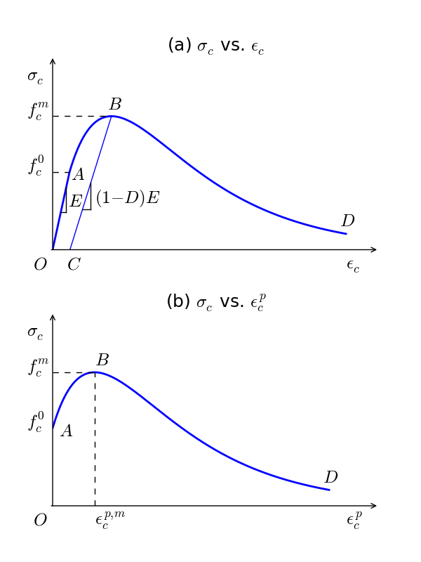
Figure 1: Typical uniaxial compression curves: top - uniaxial compressive stress vs compressive strain; bottom - uniaxial compressive stress vs plastic compressive strain.

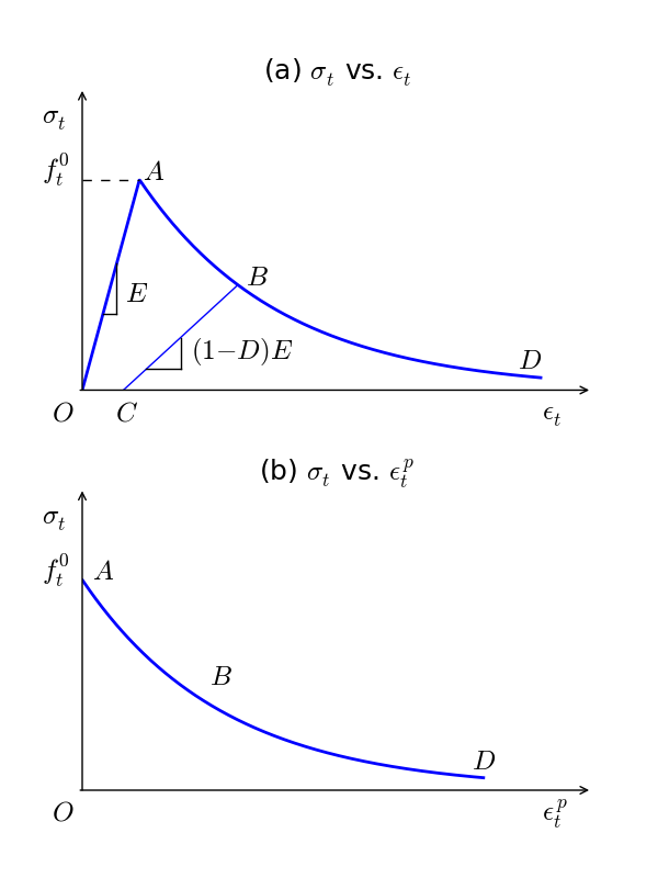
Figure 2: Typical uniaxial tension curves: top - uniaxial tensile stress vs tensile strain; bottom - uniaxial tensile stress vs plastic tensile strain.

For stress defined by Equation (3), the quantity $g_{\chi}$, which denotes the dissipated energy density during the entire process of microcracking, has a closed-form expression of the area under the curve of A-B-D in Figure 1-(b) or 2-(b):

(6) $$g_{\chi} = \int_{0}^{+\infty} {\sigma_{\chi} \, d \epsilon_{\chi}^p} = \frac{f_{\chi 0}}{b_{\chi}} \left( 1 + \frac{a_{\chi}}{2} \right)$$

The initial slope of the curve $\sigma_{\chi}$-$\epsilon_{\chi}^p$ is

(7) $$\left. \frac{d \sigma_{\chi}}{d \epsilon_{\chi}^p} \right|_{\epsilon_{\chi}^p = 0} = f_{\chi 0} b_{\chi} (a_{\chi} - 1)$$

Note that $a_{\chi} > 1$ implies initial hardening (e.g., when $\chi = c$) and $a_{\chi} < 1$ implies softening immediately after yielding (e.g., when $\chi = t$). When $a_{\chi} > 1$, $\sigma_{\chi}$ obtain a maximum value (see Point A in Figure 1)

(8) $$f_{\chi}^m = f_{\chi 0} \frac{(1+a_{\chi})^2}{4a_{\chi}}$$

at

(9) $$\epsilon_{\chi}^{p,m} = - \frac{\ln{\left(\frac{1+a_{\chi}}{2a_{\chi}}\right)}}{b_{\chi}}$$

For a curve with initial hardening after yielding which is typical in uniaxial compression, the material constant $a_{\chi}$ can be back-calculated from Equation (8) by

(10) $$a_{\chi} = 2 (f_{\chi}^m/f_{\chi 0}) - 1 + 2 \sqrt{(f_{\chi}^m/f_{\chi 0})^2 - (f_{\chi}^m/f_{\chi 0})}$$

For a curve with immediate softening after yielding which is typical in uniaxial extension, a simple way is assuming $a_t = 0$, which leads to

(11) $$\sigma_t = f_{t0} \exp{(-b_t \epsilon_t^p)}$$

and

(12) $$g_t = f_{t0} / b_t$$

Once $a_{\chi}$ is determined or assumed, $b_{\chi}$ can be obtained from Equation (6) provided $g_{\chi}$ and $f_{\chi 0}$ are known.

Because the capacity for the dissipated energy per unit volume cannot be given as a material property, $g_{\chi}$ should be derived from other known material properties such as the fracture energy (Lee & Fenvas, 1998). Assuming that the fracture energy in the uniaxial tensile state $G_{\chi}$ and its counterpart in the uniaxial compressive state are given as a material properties, $g_{\chi}$ is the specific fracture energy normalized by the localization zone size, also referred to as the characteristic length $l_{\chi}$, which leads to (Lubliner et al. 1989)

(13) $$g_{\chi} = \frac{G_{\chi}}{l_{\chi}}$$

To maintain objective results at the structural level, $l_{\chi}$ should be an objective value or assumed as a material property.

Yield Function

The yield surface is schemed by Figure Figure #model-concrete-yd in the biaxial-stress (plane-stress) space. Note that we assume the principle stresses with the order $\sigma_1 \le \sigma_2 \le \sigma_3$ and positive for tension. Due to symmetry, only A-B-C-D is considered.

For line A-B, a tension yield criteria is used:

(14) $$f^t (\bar{\sigma}) = \bar{\sigma}_3 - \bar{\sigma}_t = 0$$

For line B-C, a Mohr-Coulomb yield criteria is used:

(15) $$f^s (\bar{\sigma}) = - \bar{\sigma}_t \bar{\sigma}_1 + \bar{\sigma}_c \bar{\sigma}_3 - \bar{\sigma}_c \bar{\sigma}_t= 0$$

For curve C-D, a Drucker-Prager yield criteria is used:

(16) $$f^d (\bar{\sigma}) = \alpha \bar{I}_1 + \bar{q} - (1-\alpha) \bar{\sigma}_c = 0$$

where $\bar{I}_1$ is the first stress invariant, $\bar{q}$ is the equivalent shear stress, and

(17) $$\alpha = \frac{f_{b0}/f_{c0} - 1}{2(f_{b0}/f_{c0}) - 1}$$

where $f_{c0}$ is the uniaxial yield compressive strength and $f_{b0}$ is the biaxial yield compressive strength. Since usually $f_{b0} \ge f_{c0}$, $\alpha$ is in the range of $0 \le \alpha < 0.5$.

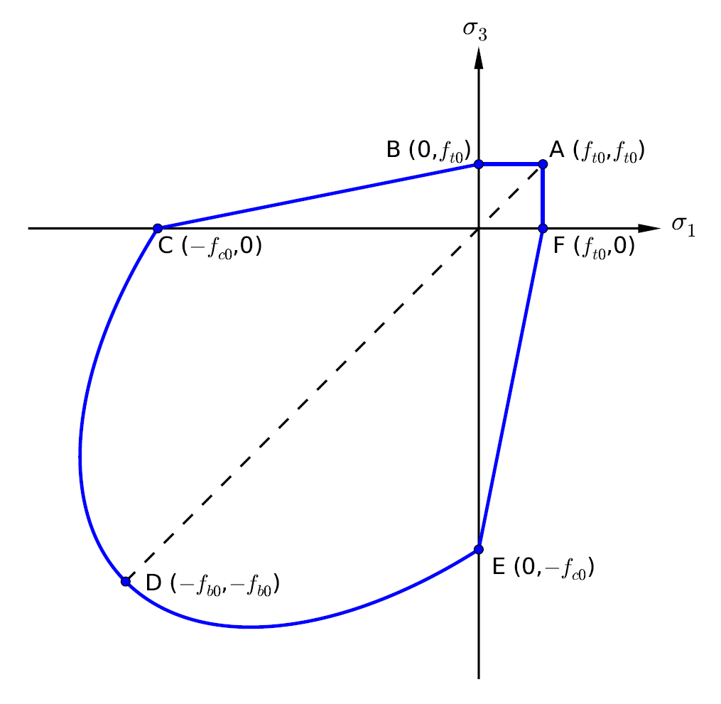
Figure 3: Schematic of initial yield surface in the biaxial-stress (plane-stress) space.

Flow Rule

The plastic strain rate is evaluated by the flow rule, which is defined by a scalar plastic potential function $g$. For a plastic potential in the effective stress space, the plastic strain is given by

(18) $$\Delta \epsilon_{ij}^p = \lambda \frac{\partial g}{\partial \bar{\sigma}_{ij}}$$

where $\lambda$ is a non-negative function referred to as the plastic consistency parameter (plastic multiplier).

For yielding at line A-B, an associated potential function is used:

(19) $$g^t (\bar{\sigma}) = \bar{\sigma}_3 - \bar{\sigma}_t$$

For yielding at line B-C, a nonassociated Mohr-Coulomb type potential function is used:

(20) $$g^s (\bar{\sigma}) = - \bar{\sigma}_1 + N_{\psi} \bar{\sigma}_3$$

where $N_{psi} = \min(\bar{\sigma}_c/\bar{\sigma}_t, (1+\sin{\psi})/(1-\sin{\psi})$ and $\psi$ is the dilation angle which is an input material property.

For yielding at curve C-D, a nonassociated Drucker-Prager yield criteria is used:

(21) $$g^d (\bar{\sigma}) = \alpha_p \bar{I}_1 + \bar{q}$$

where $\alpha_p = min(\alpha, 6\sin{\psi}/(3-\sin{\psi}))$.

Another internal variable set, besides the plastic strain, is needed to represent the damage states. The damage variable, $\kappa_{\chi}$, is assumed to be the only necessary state variable and its evolution is expressed as

(22) $$\Delta \kappa_t = r(\bar{\sigma}) \frac{f_t}{g_t} \Delta \epsilon_3^p$$

(23) $$\Delta \kappa_c = (1-r(\bar{\sigma})) \frac{f_c}{g_c} \Delta \epsilon_1^p$$

where $\epsilon_1^p$ is the minimum principal plastic strain, $\epsilon_3^p$ is the maximum principal plastic strain; $r$ is a weight function of the effective principal stresses, which ranges from 0 in pure compressive loading to 1 in pure tensile loading:

(24) $$r(\bar{\sigma}) = \frac{\sum_{i=1}^3 \langle \bar{\sigma}_i \rangle}{\sum_{i=1}^3 | \bar{\sigma}_i |}$$

Evolution of Damage

To model the different damage states for tensile and compressive loading, both $\kappa_t$ and $\kappa_c$ are used as independent damage variables. The evolution equations for the hardening and degradation variables are obtained from the factorization of the uniaxial stress strength function, $f_{\chi}=f_{\chi}(\kappa_{\chi})$, such that

(25) $$f_{\chi} = (1 - D_{\chi}) \bar{f}_{\chi}$$

in which $0 \le D_{\chi} < 1$ and $\Delta D_{\chi} > 0$. $\bar{\sigma}_{\chi} = \bar{f}_{\chi}$ describes the evolution of the cohesion variable used in the yield function, and $D_{\chi} = D_{\chi}(\kappa_{\chi})$ defines the degradation damage as a function of the damage variable:

(26) $$D = 1 - (1- D_c)(1 - sD_t)$$

where

(27) $$s = s_0 + (1 - s_0) r(\bar{\sigma})$$

with $0 \le s_0 \le 1$ and so $s_0 \le s \le 1$ represents stiffness recovery.

The degradation is also assumed an exponent form as

(28) $$1 - D_{\chi} = \exp{( - d_{\chi} \epsilon_{\chi}^p)}$$

where $d_{\chi}$ are material constants, which can be determined form the unloading-reloading (see B-C lines in Figure 1-a & 2-a).

Material Properties

In this model, two material properties, initial Young’ modulus and Poisson’s ratio, ($E$, $\nu$), or initial bulk and shear modulus, ($K$, $G$), are required to determine the elasticity.

To match the uniaxial compression and tension experimental curves, one straightforward approach is to specify the initial and peak (maximum) strengths ($f_{\chi 0}$ and $f_{\chi}^m$), fracture energies ($G_{\chi}$), characteristic lengths ($l_{\chi}$), and damages at specific stresses ($D_c^{peak}$ and $D_t^{half}$) in the uniaxial compression/tension states. These input will determine the parameters $a_{\chi}$, $b_{\chi}$, $d_{\chi}$ and $g_{\chi}$.

Once $f_{\chi 0}$ and $f_{\chi}^m$ are known, there are two cases:

• if the curve is hardening and then softening (usually in uniaxial compression experiments, see Figure 1), or in other words, $f_{\chi}^m > f_{\chi 0}$, then $a_{\chi}$ can be determined by Equation (10).

• if the curve is immediately softening (usually in uniaxial extension experiments, see Figure 2), or in other words, $f_{\chi}^m = f_{\chi 0}$, then $a_{\chi}$ will be assumed zero.

Once $G_{\chi}$ and $l_{\chi}$ are known, then $g_{\chi} = G_{\chi}/l_{\chi}$, $b_{\chi}$ can then be determined by Equation (6) so that $b_{\chi}=f_{\chi 0}(1+a_{\chi}/2)/g_{\chi}$.

Equation (28) can determine $d_{\chi}$:

• for uniaxial compression where the curve is hardening and then softening, then $d_c$ can be calculated by the the damage at the peak stress,

(29) $$d_c = b_c \frac{\ln{(1-D_c^{peak})}}{\ln{\left( \frac{1+a_c}{2a_c} \right)}}$$

• for uniaxial extension where the curve is immediately softening, then $d_t$ can be calculated by the the damage at the half peak/initial stress,

(30) $$d_t = b_t \frac{\ln{(1-D_t^{half})}}{-\ln{2}}$$

$\alpha_p$ is a material property determining the dilation, with typical value $\alpha_p=0.2$.

The biaxial compression initial strength $f_{b0}$ is requited to calculate $\alpha$ in Equation (17). Here the ratio $f_{b0}/f_{c0}$ is instead as an input material property, with a typical value $f_{b0}/f_{c0} = 1.05{\sim}1.2$.

The stiffness recovery parameter $s_0$ is usually in the range of $0 \le s_0 \le 0.2$.

References

Lee, J., & Fenves, G. L. (1998). Plastic-damage model for cyclic loading of concrete structures. Journal of engineering mechanics, 124(8), 892-900.

Lee, J., & Fenves, G. L. (1998). A plastic damage concrete model for earthquake analysis of dams. Earthquake engineering & structural dynamics, 27(9), 937-956.

Lubliner, J., Oliver, J., Oller, S., & Onate, E. (1989). A plastic-damage model for concrete. International Journal of solids and structures, 25(3), 299-326.

concrete Model Properties

Use the following keywords with the zone property command to set these properties of the concrete model.

concrete

bulk f

bulk modulus, $K$.

compression-strength f

uniaxial compression peak/maximum strength, $f_c^m$.

compression-initial f

uniaxial compression initial yield strength, $f_{c0}$.

compression-energy-fracture f

fracture energy in uniaxial compression state, $G_c$.

compression-length-reference f

reference (characteristic) length in uniaxial compression state, $l_c$.

compression-d f

compression damage parameter, $d_c$.

dilation f

dilation angle, $\psi$.

poisson f

Poisson’s ratio, $\nu$.

ratio-biaxial f

strength ratio of biaxial to uniaxial compression initial, usually in a range of (1,1.25], $f_{b0}/f_{c0}$.

shear f

shear modulus, $G$.

tension-strength f

uniaxial tension peak/maximum strength, $f_t^m$.

tension-initial f

uniaxial tension initial yield strength, $f_{t0}$. Usually, $f_{t0} = f_t^m$.

tension-energy-fracture f

fracture energy in uniaxial compression state, $G_t$.

tension-length-reference f

reference (characteristic) length in uniaxial tension state, $l_t$.

tension-d f

tension damage parameter, $d_t$.

tension-recovery f

stiffness recovery parameter for tension, typical value is 0.2, $s_0$.

young f

Young’s modulus, $E$.

compression f (r)

Current compression strength, $\sigma_c$.

damage f (r)

Current total damage, $D$.

damage-compression f (r)

Current damage in compression, $D_c$.

damage-tension f (r)

Current damage in tension, $D_t$.

strain-plastic-compression f (r)

Current plastic strain in compression, $\epsilon^p_c$.

strain-plastic-tension f (r)

Current plastic strain in tension, $\epsilon^p_t$.

tension f (r)

Current tension strength, $\sigma_t$.

Notes

• Only one of the two options is required to define the elasticity: bulk modulus $K$ and shear modulus $G$, or, Young’s modulus $E$ and Poisson’s ratio $\nu$. When choosing the latter, Young’s modulus $E$ must be assigned in advance of Poisson’s ratio $\nu$.

Key

(a) Advanced property.

This property has a default value; simpler applications of the model do not need to provide a value for it.

(r) Read-only property.

This property cannot be set by the user. Instead, it can be listed, plotted, or accessed through FISH.