Elastic Plate (Orthotropic) with Uniform Lateral Load

Problem Statement

Note

To view this project in FLAC3D, use the menu command Help ► Examples…. Choose “Structure/Shell/Orthotropic” and select “Orthotropic.prj” to load. The main data files are shown at the end of this example. The remaining data files can be found in the project.

The displacement field, bending and transverse-shear stress resultants for a simply supported rectangular elastic plate with an orthotropic elastic constitutive model are computed and compared with the analytical solution. The plate is modeled both with and without stiffeners. The procedure to compute the rigidities is explained; it consists of constructing an orthotropic plate with elastic properties equal to the average properties of the components of the original plate. The rigidities are used, along with the plate thickness, to compute the orthotropic bending elastic constants that must be specified for the orthotropic elastic constitutive model. This problem tests the orthotropic elastic constitutive model, and quantifies the ability of the DKT element to model the bending action.

Analytical Solution

A simply supported rectangular plate (with side lengths \((a)\) and \((b)\)) is subjected to a uniform lateral load \((p_o)\). The plate has an orthotropic elastic material model. The analytical solution for lateral deflection as well as bending and transverse-shear stress resultants is given by Ugural (1981, Section 6.4). The load is resisted by bending action, and thus, the membrane stress resultants are zero. The analytical solution is expressed via the notation in Figure 1 in which the principal directions of orthotropy are aligned with the \(x\) and \(y\) axes.

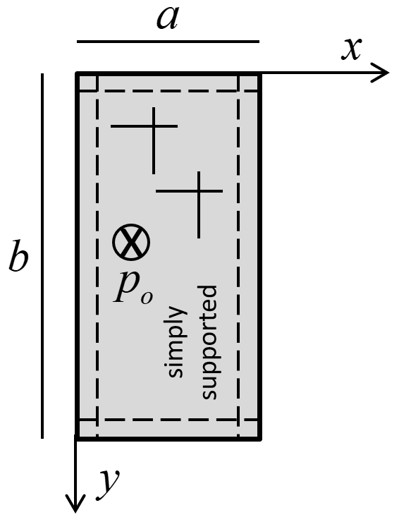
Figure 1: Rectangular plate, lateral loading, directions of orthotropy and coordinate system used to express the analytical solution.

The lateral deflection is given by

\[\begin{split}\begin{align} w &= \frac{16 p_o}{\pi^6} \sum_m^\infty \sum_n^\infty \frac{\sin(m \pi x / a) \sin(n \pi y / b)}{\beta} \\ \beta &= m n \Bigl[ D_x ( m/a )^4 + 2H ( mn/ab )^2 + D_y ( n/b )^4 \Bigr] \\ H &= D_{xy} + 2 G_{xy} \\ &\qquad\qquad\qquad (m,n = 1,3,\dots) \end{align}\end{split}\]

where \(p_o\) is uniform lateral load; \(a\) is length in the \(x\) direction; \(b\) is length in the \(y\) direction; \(D_x\), \(D_y\) and \(D_{xy}\) are flexural rigidities; \(G_{xy}\) is torsional rigidity; and \(t\) is plate thickness. The solution reduces to that of an isotropic elastic plate by expressing the rigidities in terms of the isotropic elastic constants:

(1)\[\begin{split}\begin{gather} D_x = D_y = H = D = {Et^3 \over 12(1-\nu^2)}, \quad D_{xy} = \nu D \\ G_{xy} = D(1 - \nu)/2 \end{gather}\end{split}\]

where \(E\) is Young’s modulus and \(\nu\) is Poisson’s ratio.

The bending stress resultants are

\[\begin{split}\begin{align} M_x &= -\left( D_x \frac{\partial^2 w}{\partial x^2} + D_{xy} \frac{\partial^2 w}{\partial y^2} \right) \\ M_y &= -\left( D_y \frac{\partial^2 w}{\partial y^2} + D_{xy} \frac{\partial^2 w}{\partial x^2} \right) \\ M_{xy} &= -2 G_{xy} \frac{\partial^2 w}{\partial x \partial y} \end{align}\end{split}\]

which can be expressed as

\[\begin{split}\begin{align} M_x &= \frac{16 p_o}{\pi^4} \sum_m^\infty \sum_n^\infty \left[ \frac{D_x (m/a)^2 + D_{xy} (n/b)^2}{\beta} \right] \sin(m \pi x / a) \sin(n \pi y / b) \\ M_y &= \frac{16 p_o}{\pi^4} \sum_m^\infty \sum_n^\infty \left[ \frac{D_{xy} (m/a)^2 + D_y (n/b)^2}{\beta} \right] \sin(m \pi x / a) \sin(n \pi y / b) \\ M_{xy} &= -\frac{16 p_o}{\pi^4} \sum_m^\infty \sum_n^\infty \left[ \frac{2 G_{xy} (mn/ab) }{\beta} \right] \cos(m \pi x / a) \cos(n \pi y / b) \\ &\qquad(m,n = 1,3,\dots) \end{align}\end{split}\]

The transverse-shear stress resultants are

\[\begin{split}\begin{align} Q_x &= -\frac{\partial}{\partial x} \left( D_x \frac{\partial^2 w}{\partial x^2} + H \frac{\partial^2 w}{\partial y^2} \right) \\ Q_y &= -\frac{\partial}{\partial y} \left( D_y \frac{\partial^2 w}{\partial y^2} + H \frac{\partial^2 w}{\partial x^2} \right) \end{align}\end{split}\]

which can be expressed as

\[\begin{split}\begin{align} Q_x &= \frac{16 p_o}{\pi^3} \sum_m^\infty \sum_n^\infty \left[ \frac{D_x (m/a)^3 + H (mn^2/ab^2)}{\beta} \right] \cos(m \pi x / a) \sin(n \pi y / b) \\ Q_y &= \frac{16 p_o}{\pi^3} \sum_m^\infty \sum_n^\infty \left[ \frac{D_y (n/b)^3 + H (m^2n/a^2b)}{\beta} \right] \sin(m \pi x / a) \cos(n \pi y / b) \\ &\qquad (m,n = 1,3,\dots) \end{align}\end{split}\]

Particular Problem

The particular problem to be considered is defined as follows. Consider a 4 by 8 sheet of three-quarter inch plywood that is simply supported along its edges, and stiffened with a set of three equally spaced 2 by 4 boards that are attached such that no slip can occur at the interface between the boards and the sheet as shown in Figure 2.

Figure 2: Plywood sheet stiffened with 2 by 4 boards.

The problem geometry is defined by the properties:

\[\begin{split}\begin{gather} t = 19 \textrm{ mm}, \quad a = 2440 \textrm{ mm}, \quad b = 1220 \textrm{ mm} \\ s = 407 \textrm{ mm}, \quad w = 38 \textrm{ mm}, \quad h = 89 \textrm{ mm} \\ \bigl[ \textrm{thin plate: }a/t > 20 \bigr] \end{gather}\end{split}\]

The plywood sheet and 2 by 4 boards are assumed to behave as isotropic elastic materials[1]:

\[E = 8.5 \textrm{ GPa}, \quad \nu = 0.33\]

A box of dry sand that is one-half meter deep sits on top of the plywood sheet, inducing a uniform lateral load:

\[\begin{split}\begin{gather} p_o = \rho g H = 7.86 \textrm{ kPa} \\ \bigl[ \rho = 1602 \textrm{ kg} / \textrm{m}^3,\ g = 9.81 \textrm{ m} / \textrm{s}^2,\ H = 0.5 \textrm{ m} \bigr] \end{gather}\end{split}\]

Computing Rigidities

The analytical solution is expressed in terms of the four rigidities: \(D_x\), \(D_y\), \(D_{xy}\) and \(G_{xy}\). For the unstiffened sheet, the rigidities are expressed in terms of \(E\) and \(\nu\) via Eq. (1). For the stiffened sheet, the rigidities are computed by constructing an orthotropic plate with elastic properties equal to the average properties of the components of the original plate. This is done using the relations for the case of a plate reinforced by a set of equidistant ribs in Ugural (1981, Table 6.1) — shown here:

\[\begin{split}\begin{align} D_x &= \frac{E s t^3} {12 \left[ s - w + w \left( \frac{t}{h + t} \right)^3 \right]} \\ D_y &= \frac{EI}{s} \\ D_{xy} &= 0 \\ G_{xy} &= \tfrac{1}{2} \left( H - D_{xy} \right), \quad H = 2 G\,'_{xy} + \frac{C}{s} \end{align}\end{split}\]

where \(G\,'_{xy}\) is torsional rigidity of the sheet; \(C\) is torsional rigidity of one rib; \(I\) is moment of inertia about neutral axis of the T-section shown in Figure 3; and \(E\) is elastic modulus of the sheet. The first three terms are obtained as follows.

The first term:

\[G\,'_{xy} = \frac{Gt^3}{12}, \quad G = \frac{E}{2(1 + \nu)}\]

The second term:

\[\begin{split}\begin{gather} C = c_2 h w^3 G \\ \left[ c_2 = 0.241 - \textrm{Crandall et al. (1978, Table 6.1) } \right] \end{gather}\end{split}\]

The third term:

\[\begin{split}\begin{gather} I = \tfrac{1}{12} s t^3 + \left( h + t/2 - \bar{y} \right)^2 s t + \tfrac{1}{12} w h^3 + \left( \bar{y} - h/2 \right)^2 w h \\ \bar{y} = \frac{(t + 2h) st + wh^2}{2(st + wh)} \end{gather}\end{split}\]

The rigidities for the stiffened sheet have the values:

\[\begin{split}\begin{align} D_x & = 5.36\times10^3 \textrm{ Nm} \\ D_y & = 195\times10^3 \textrm{ Nm} \\ D_{xy} &= 0 \\ G_{xy} &= 6.45\times10^3 \textrm{ Nm} \end{align}\end{split}\]

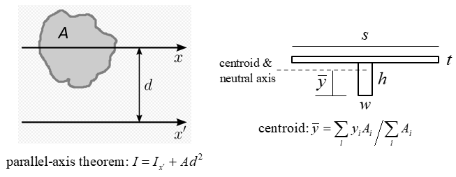
Figure 3: Computing geometric properties of a stiffener.

FLAC3D Models

The sheet is modeled using a 16 by 8 mesh of DKT elements with a cross-diagonal pattern as shown in Figure 4. The cross-diagonal pattern is used to ensure symmetric response. The orthotropic elastic constitutive model is used for both the unstiffened and stiffened cases.[2] The principal directions of orthotropy are aligned with the global \(x\) and \(y\) axes; the material coordinate system defines these directions and is specified as shown here. The orthotropic bending elastic constants are obtained from the rigidities using these relations. The orthotropic elastic membrane elastic constants are not required, because the load is resisted by bending action only. The simply-supported boundary condition (translational velocity fixed in the \(z\) direction) is assigned to the nodes along the plate edges. The lateral load is applied over the plate surface as a uniform pressure acting in the positive \(z\) direction. The \(z\)-displacement at the plate center is monitored as a history. Local nonviscous damping is used with a damping factor of 0.8. The models are run in small-strain mode to correspond with the small-strain assumption of the analytical solution. The models are cycled until a convergence limit of \(1 \times 10^{-3}\) is achieved. The model response is compared with the analytical solution along various lines. The analytical values are obtained by taking the first 50 terms \((m \leq 100, n \leq 100)\) of the infinite series.

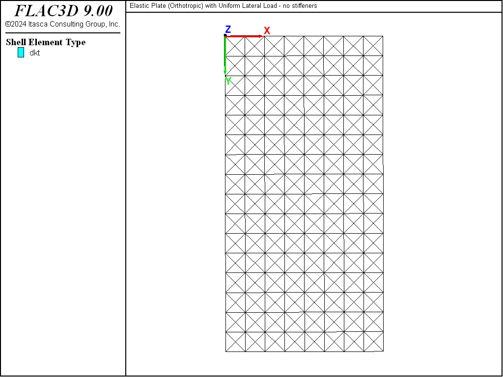
Figure 4: Geometry of the FLAC3D model showing mesh and global coordinate system.

Results and Discussion

The deformed shapes and center-deflection histories for the two cases are shown in Figures 5 and 6, from which we conclude that the static solutions have been obtained. The stiffeners reduce the plate deflection from approximately 32 to 12 mm.

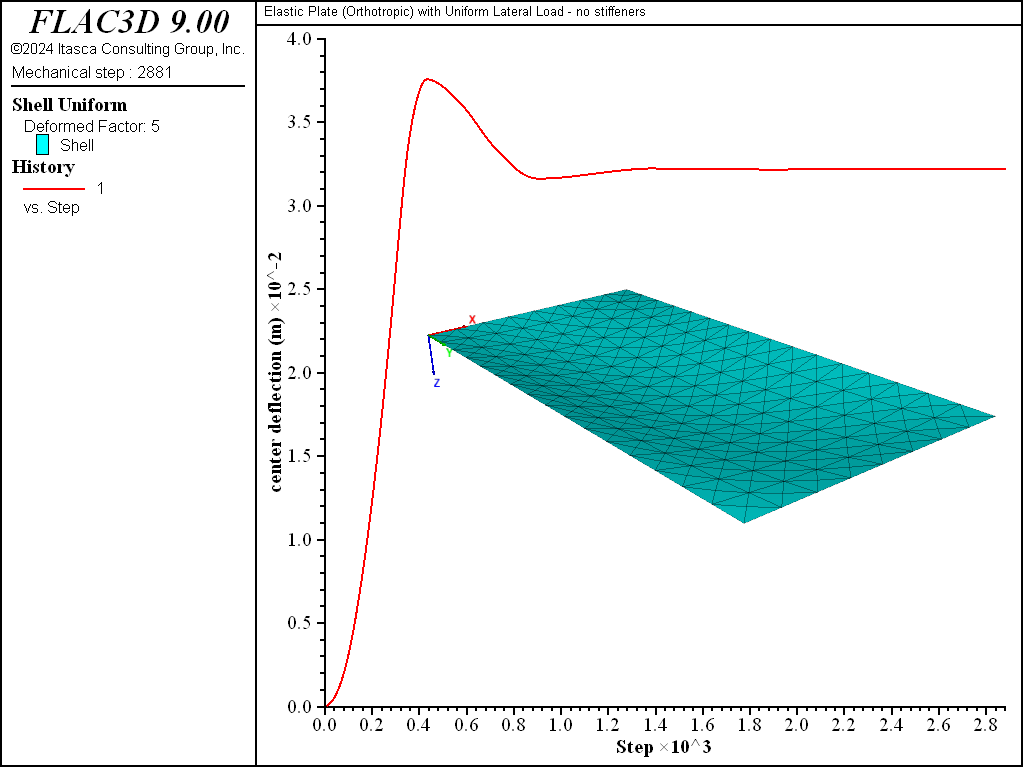
Figure 5: Deformed shape (deformation factor: 5) and center deflection (no stiffeners).

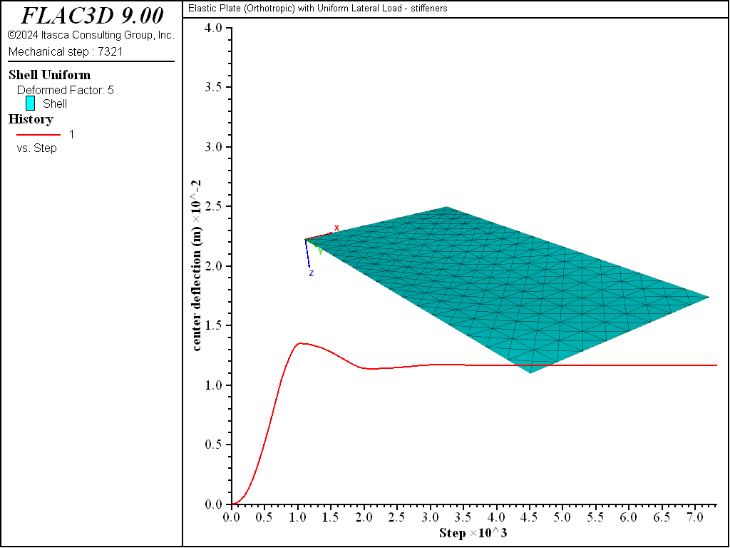
Figure 6: Deformed shape (deformation factor: 5) and center deflection (stiffeners).

The lateral deflection is obtained from the \(z\) displacement of the nodes along the indicated line. The lateral deflection along the \(x = a/2\) line for the two cases is shown in Figures 7 and 8. The computed deflections are within 1.5% of the analytical values at all sampling locations.

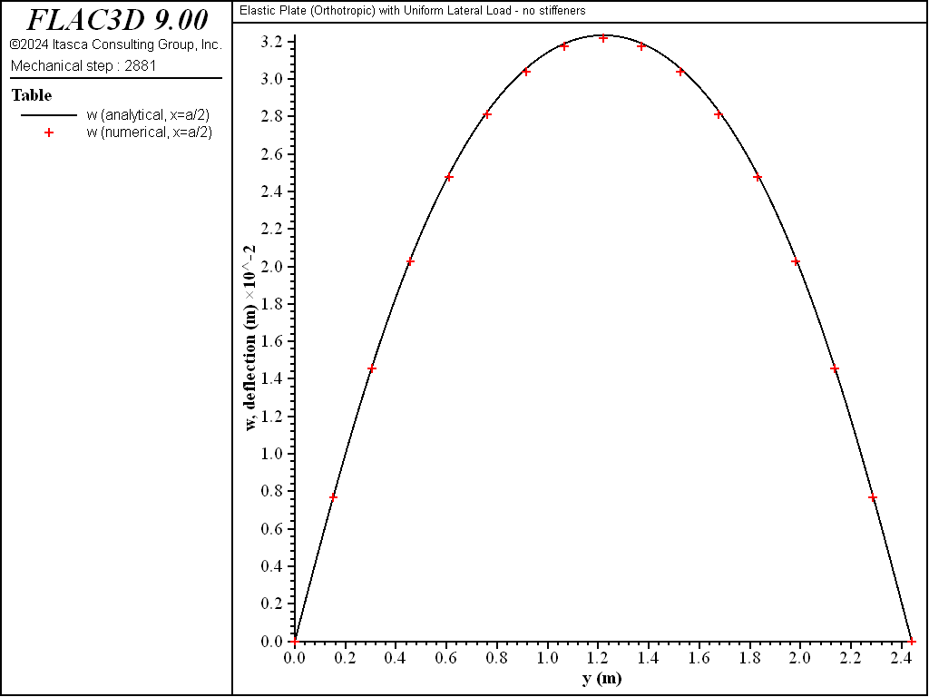
Figure 7: Lateral deflection along the \(x = a/2\) line (no stiffeners)

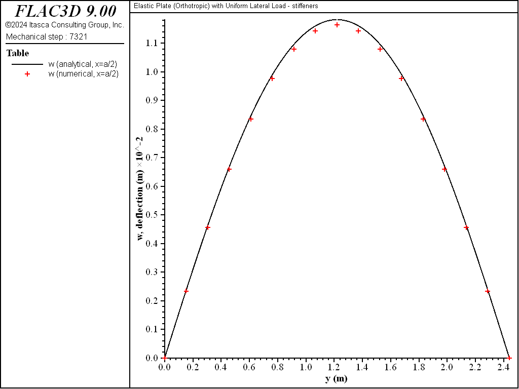
Figure 8: Lateral deflection along the \(x = a/2\) line (stiffeners)

The stress resultants are expressed in a surface coordinate system that is aligned with the global coordinate system. The bending stress resultants are obtained at the nodes along the indicated line — these values have been averaged for the shell elements that share each node. The transverse-shear stress resultants are obtained at the centroids of the shell elements just to the side of the indicated line — there is no averaging at nodes. The stress resultant field variations are displayed as contours using the Structural Element:Shell plot item, and checking the Use Engine Data box (discussed here).

The \(M_x\) stress resultant along the \(x = a/2\) line for the two cases is shown in Figures 9 and 10. The computed values are within 1.2% of the analytical values at all sampling locations where the analytical values are not zero. The values at the ends are not zero, but will approach zero as the mesh is refined.

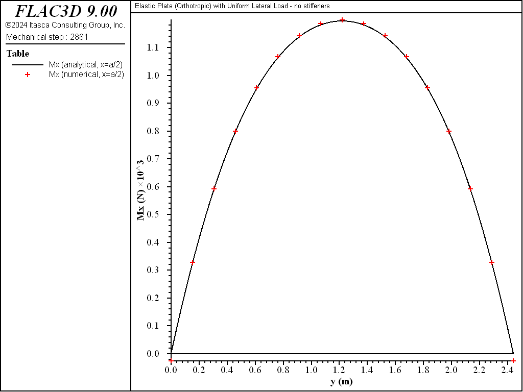
Figure 9: \(M_x\) stress resultant along the \(x = a/2\) line (no stiffeners).

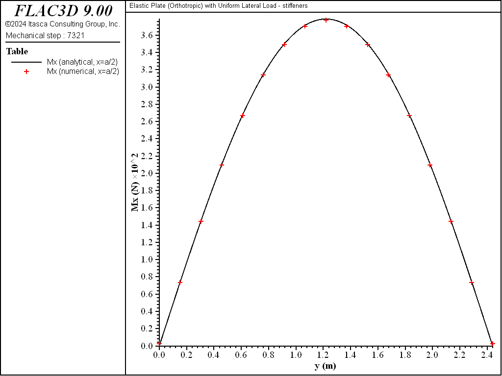
Figure 10: \(M_x\) stress resultant along the \(x = a/2\) line (stiffeners).

The variation of the \(M_y\) stress resultant over the sheet surface for the two cases is shown in Figures 11 and 12. The \(M_y\) stress resultant along the \(x = a/2\) line for the two cases is shown in Figures 13 and 14. The computed values are within 1.8% of the analytical values at all sampling locations where the analytical values are not zero. The values at the ends are not zero, but will approach zero as the mesh is refined.

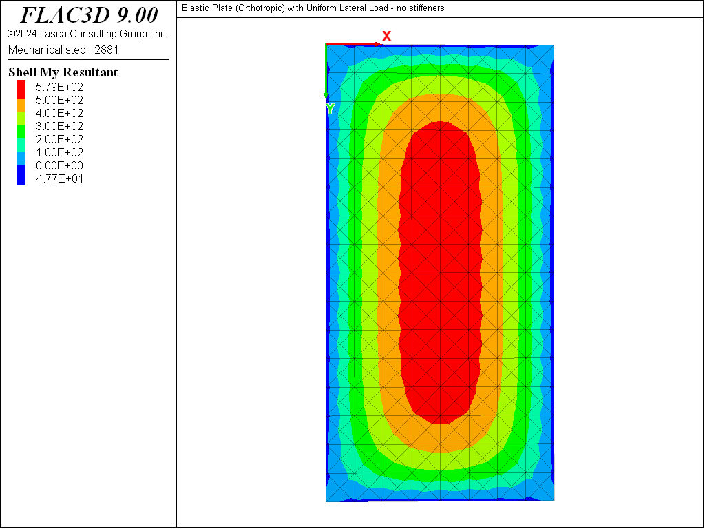
Figure 11: Variation of the \(M_y\) stress resultant over the sheet surface (no stiffeners).

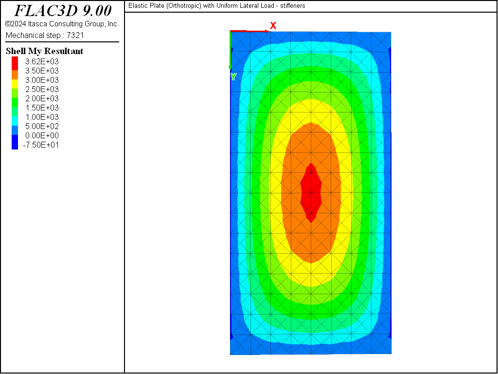
Figure 12: Variation of the \(M_y\) stress resultant over the sheet surface (stiffeners).

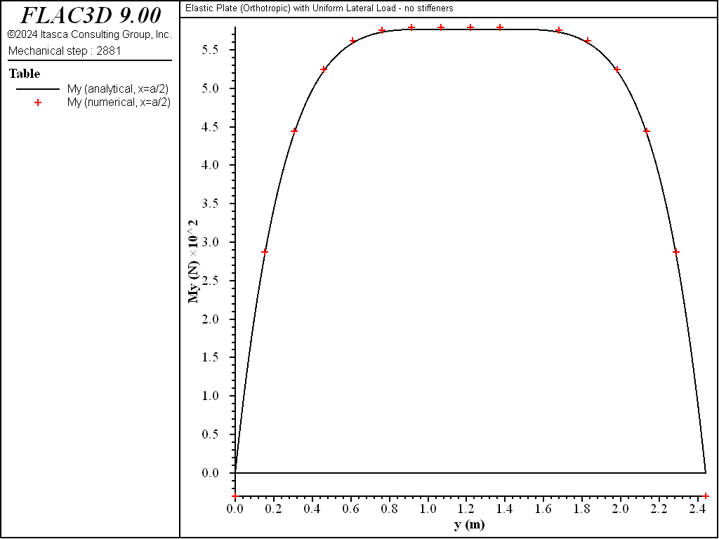
Figure 13: \(M_y\) stress resultant along the \(x = a/2\) line (no stiffeners).

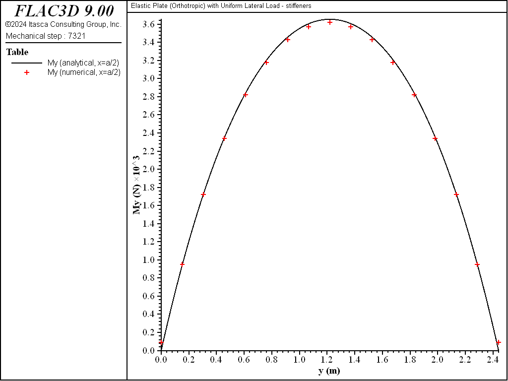
Figure 14: \(M_y\) stress resultant along the \(x = a/2\) line (stiffeners).

The variation of the \(M_{xy}\) stress resultant over the sheet surface for the two cases is shown in Figures 15 and 16. The \(M_{xy}\) stress resultant along the \(x = a/8\) line for the two cases is shown in Figures 17 and 18. The computed values are within 2.5% of the analytical values.

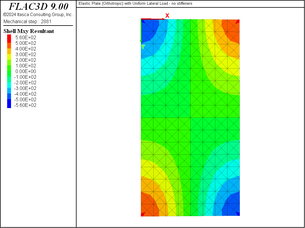
Figure 15: Variation of the \(M_{xy}\) stress resultant over the sheet surface (no stiffeners).

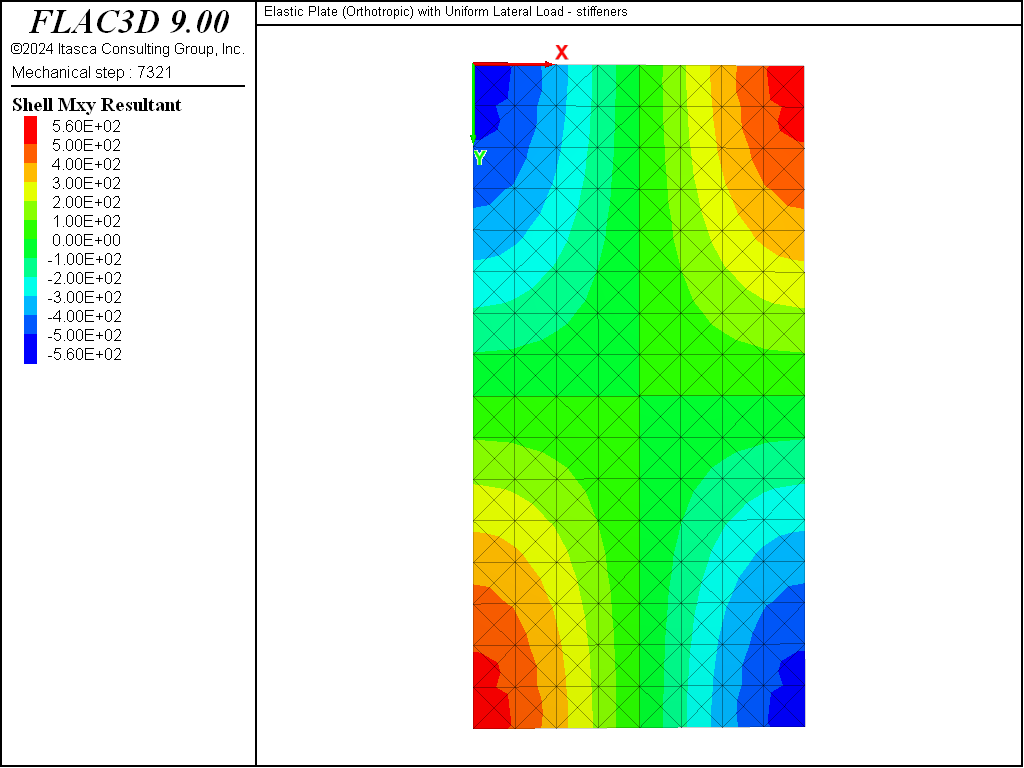
Figure 16: Variation of the \(M_{xy}\) stress resultant over the sheet surface (stiffeners).

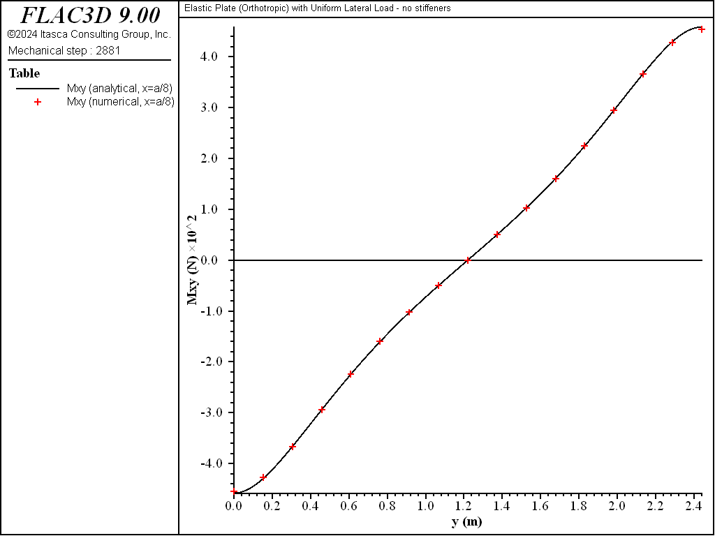
Figure 17: \(M_{xy}\) stress resultant along the \(x = a/8\) line (no stiffeners).

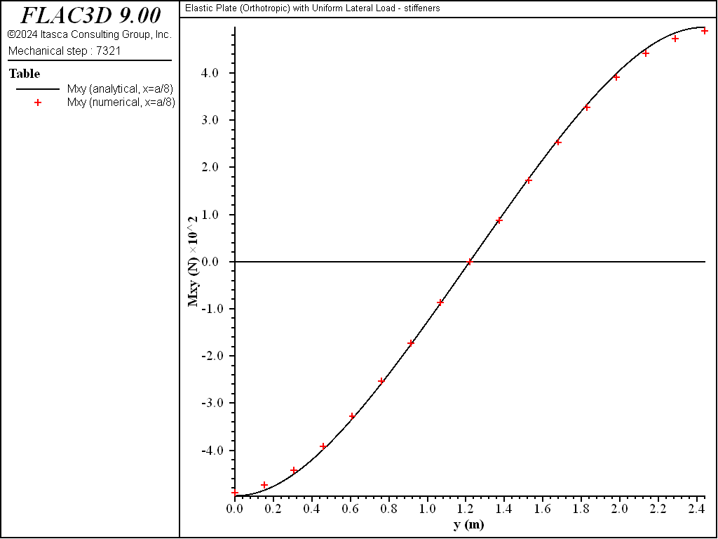
Figure 18: \(M_{xy}\) stress resultant along the \(x = a/8\) line (stiffeners).

The \(Q_x\) stress resultant along the \(y = b/2\) line for the two cases is shown in Figures 19 and 20. The computed values are within 6.2% of the analytical values. The transverse-shear stress resultants are computed with less accuracy than the bending stress resultants because the transverse-shear stress resultants are obtained from the spatial derivatives of the bending stress resultants (as shown here) — taking spatial derivatives reduces accuracy.

Figure 19: \(Q_x\) stress resultant along the \(y = b/2\) line (no stiffeners).

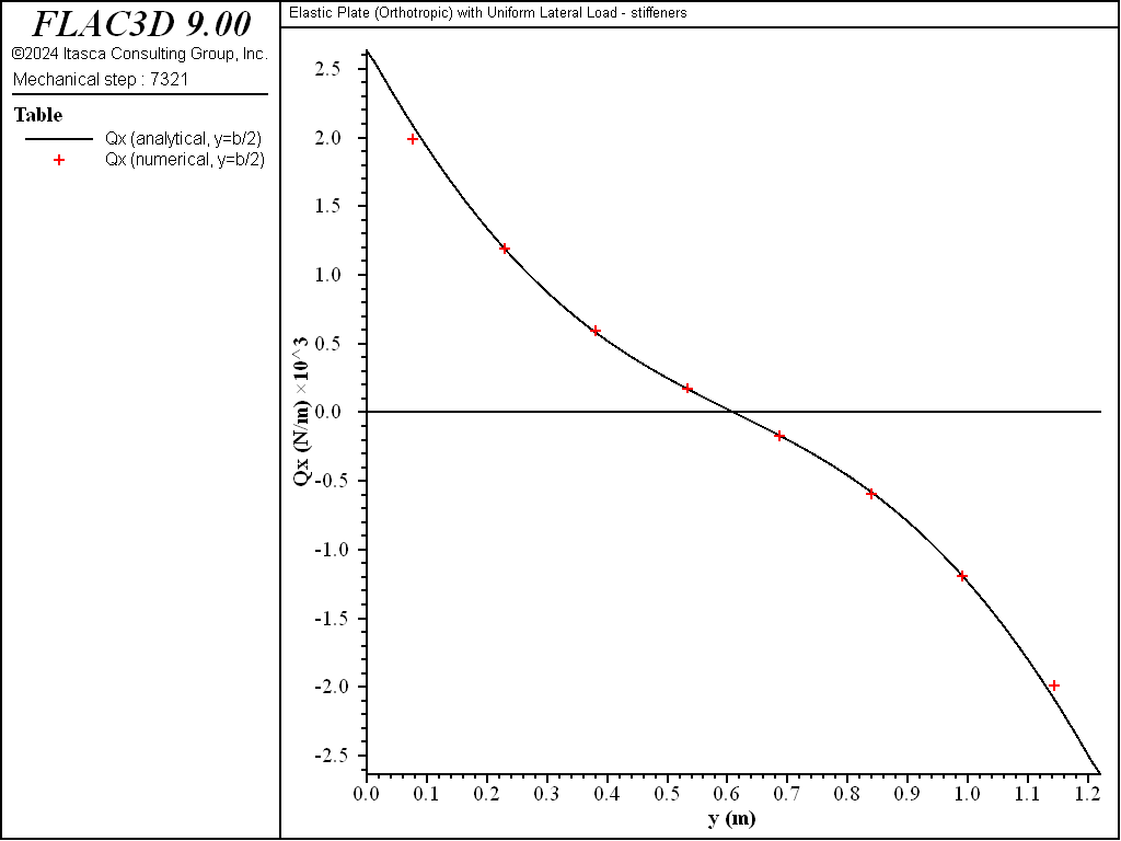
Figure 20: \(Q_x\) stress resultant along the \(y = b/2\) line (stiffeners).

The variation of the \(Q_y\) stress resultant over the sheet surface for the two cases is shown in Figures 21 and 22. The \(Q_y\) stress resultant along the \(x = a/2\) line for the two cases is shown in Figures 23 and 24. The computed values are within 8.1% of the analytical values at all sampling locations. The transverse-shear stress resultants are computed with less accuracy than the bending stress resultants because the transverse-shear stress resultants are obtained from the spatial derivatives of the bending stress resultants (as shown here) — taking spatial derivatives reduces accuracy.

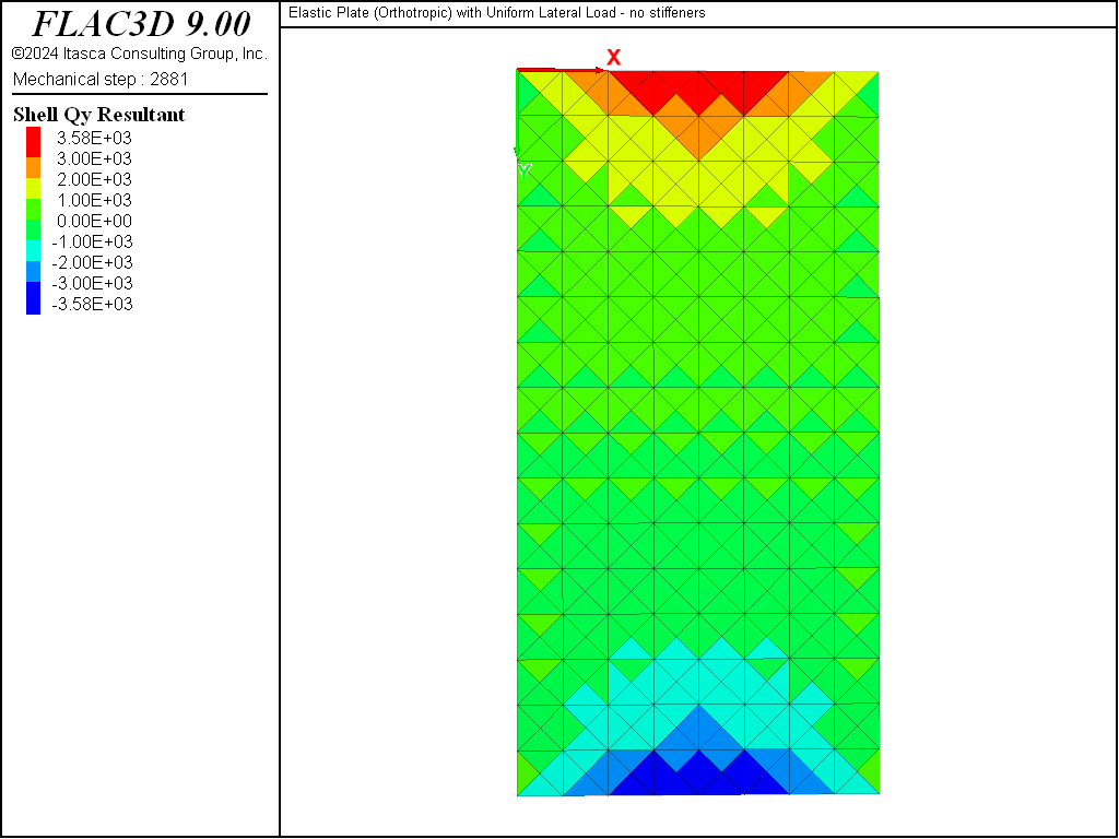
Figure 21: Variation of the \(Q_y\) stress resultant over the sheet surface (no stiffeners).

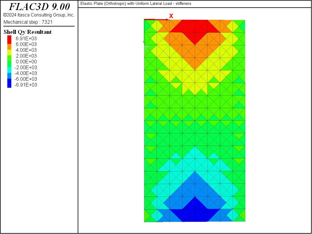
Figure 22: Variation of the \(Q_y\) stress resultant over the sheet surface (stiffeners).

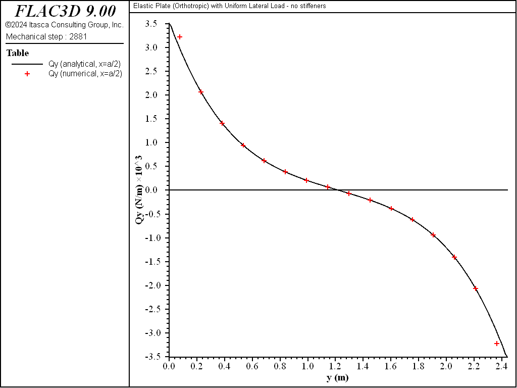
Figure 23: \(Q_y\) stress resultant along the \(x = a/2\) line (no stiffeners).

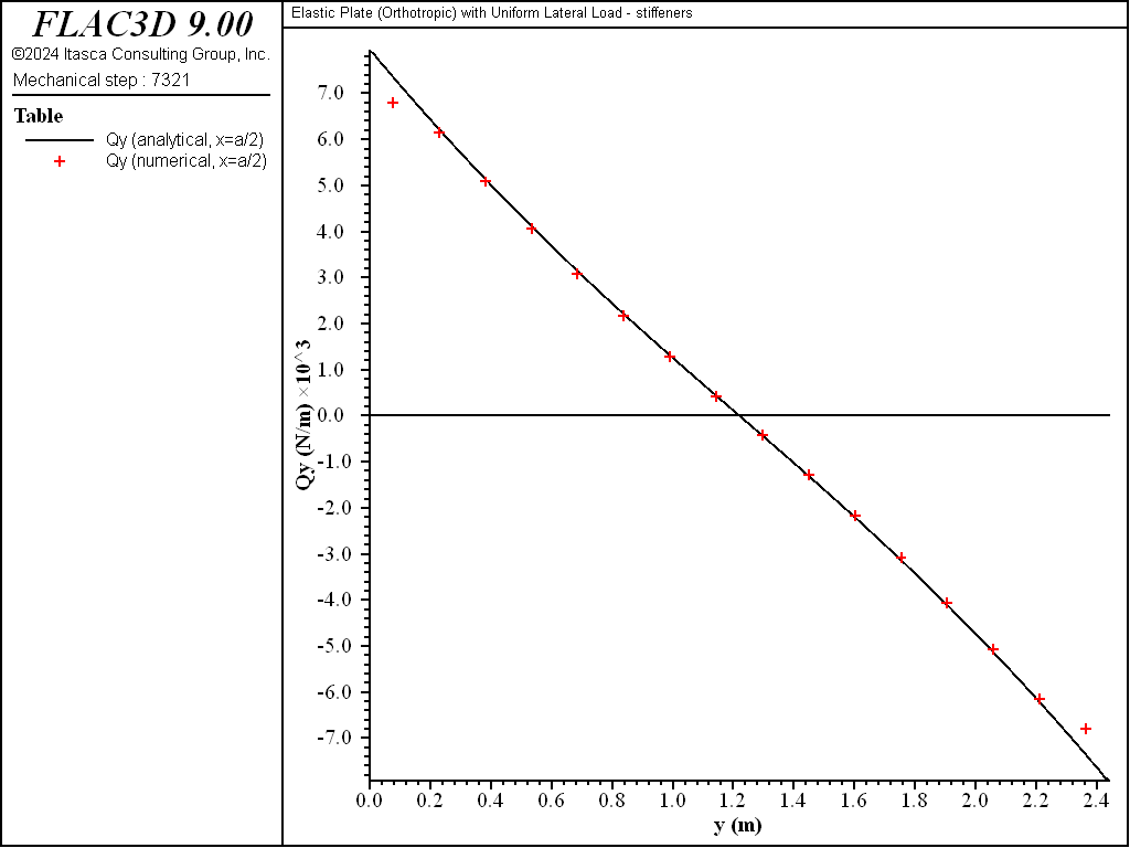
Figure 24: \(Q_y\) stress resultant along the \(x = a/2\) line (stiffeners).

References

Crandall, S.H., N.C. Dahl and T.J. Lardner. An Introduction to the Mechanics of Solids, Second Edition, New York: McGraw-Hill Book Company (1978).

Ugural, A. C. Stresses in Plates and Shells, New York: McGraw-Hill Publishing Company, Inc. (1981).

Endnotes

[1]

An improved model would consider the plywood sheet and 2 by 4 boards themselves to behave as orthotropic materials. Such an improvement is beyond the scope of this verification problem.

[2]

The unstiffened sheet could be modeled with the isotropic elastic constitutive model. Instead, it is modeled with the orthotropic elastic constitutive model, and the rigidities are expressed in terms of \(E\) and \(\nu\) via Eq. (1).

Data Files

NoStiffeners.dat

model new
fish automatic-create off
[global t = 'Elastic Plate (Orthotropic) with Uniform Lateral Load']
model title [t + ' - no stiffeners']
; =============================================================================
; Material properties, dimensions and loading (SI units)
  [global E  = 8.5e9]  ; plywood
  [global nu = 0.33]
  [global t =   19e-3] ; ~ 3/4 inch
  [global a = 1220e-3] ; 4 by 8 sheet
  [global b = 2440e-3]
  [global rho = 1602]  ; dry sand
  [global Ht = 500e-3] ; height of sand
; Derived items
  [global p0 = rho * 9.81 * Ht] ; units: N/m*m
  [global D = E*t*t*t/(12 * (1 - nu*nu))
  [global Dx = D]
  [global Dy = D]
  [global Dxy = nu*D]
  [global Gxy = 0.5*(1.0 - nu)*D]
  [global c11b = (12/(t*t*t))*Dx]
  [global c22b = (12/(t*t*t))*Dy]
  [global c12b = (12/(t*t*t))*Dxy]
  [global c33b = (12/(t*t*t))*Gxy]
; Mesh properties
  [global nx =  8]  ; should be even
  [global ny = 16]  ; should be even
; =============================================================================
; Create mesh, assign shell properties and boundary conditions.
structure shell create by-quadrilateral (0,0,0) ([a],0,0) ([a],[b],0) (0,[b],0) ...
                    size [nx] [ny]  cross-diagonal  true element-type dkt
structure shell property thickness [t]
structure shell cmodel assign orthotropic
structure shell property ortho-bend-constants [c11b] [c12b] [c22b] [c33b] ...
                      material-x 1 0 0 ; align with the global x and y direcs.

structure node fix velocity-z range position-y 0.0 position-y [b] ...
                                 position-x 0.0 position-x [a] union
structure shell apply [p0]

structure node history displacement-z position [0.5*a] [0.5*b] 0  ; plate center

model large-strain false
structure mechanical damping local 0.8
model solve convergence 1e-3

structure shell recover surface 1 0 0 ; align with the global x and y direcs.
structure shell recover resultants

model save 'NoStiffeners'

Stiffeners.dat

model new
fish automatic-create off
[global t = 'Elastic Plate (Orthotropic) with Uniform Lateral Load']
model title [t + ' - stiffeners']
; =====================================================================
; Material properties, dimensions and loading (SI units)
  [global t =   19e-3] ; ~ 3/4 inch
  [global a = 1220e-3] ; 4 by 8 sheet
  [global b = 2440e-3]
  [global rho = 1602]  ; dry sand
  [global Ht = 500e-3] ; height of sand
  [global Dx = 5.36e3]
  [global Dy = 195e3]
  [global Dxy = 0.0]
  [global Gxy = 6.45e3]
; Derived items
  [global p0 = rho * 9.81 * Ht] ; units: N/m*m
  [global c11b = (12/(t*t*t))*Dx]
  [global c22b = (12/(t*t*t))*Dy]
  [global c12b = (12/(t*t*t))*Dxy]
  [global c33b = (12/(t*t*t))*Gxy]
; Mesh properties
  [global nx =  8]  ; should be even
  [global ny = 16]  ; should be even
; =====================================================================
; Create mesh, assign shell properties and boundary conditions.
structure shell create by-quadrilateral (0,0,0) ([a],0,0) ([a],[b],0) (0,[b],0) ...
                    size [nx] [ny]  cross-diagonal  true element-type dkt
structure shell property thickness [t]
structure shell cmodel assign orthotropic
structure shell property ortho-bend-constants [c11b] [c12b] [c22b] [c33b] ...
                      material-x 1 0 0 ; align with the global x and y direcs.

structure node fix velocity-z range position-y 0.0 position-y [b] ...
                                 position-x 0.0 position-x [a] union
structure shell apply [p0]

structure node history displacement-z position [0.5*a] [0.5*b] 0  ; plate center

model large-strain false
structure mechanical damping local 0.8
model solve convergence 1e-3

structure shell recover surface 1 0 0 ; align with the global x and y direcs.
structure shell recover resultants

model save 'Stiffeners'