FLAC3D Modeling • Introduction
Overview
FLAC3D is a three-dimensional explicit Lagrangian finite-volume program for engineering mechanics computation. FLAC2D is a two-dimensional version of FLAC3D and it operates under the assumption of plane-strain. The basis for both programs is the well-established numerical formulation used by Itasca’s heritage program, FLAC.[1]
FLAC2D is a continuation of FLAC. It incorporates most of its features while utilizing modern programming framework and capabilities which are now used by most of the Itasca’s codes. FLAC3D extends the analysis capability of FLAC and FLAC2D into three dimensions, simulating the behavior of three-dimensional structures built of soil, rock, or other materials that exhibit path-dependent behavior.
Materials are represented by polygonal (in 2D) or polyhedral (in 3D) elements within a two- or three-dimensional grid that is adjusted by the user to fit the shape of the object to be modeled. Each element behaves according to a prescribed linear or nonlinear stress/strain law in response to applied forces or boundary restraints. The material can yield and flow, and the grid can deform (in large-strain mode) and move with the material that is represented.
The explicit, Lagrangian calculation scheme and the mixed-discretization zoning technique used in FLAC2D and FLAC3D ensure that plastic collapse and flow are modeled very accurately. Because no matrices are formed, large three-dimensional calculations can be made without excessive memory requirements. The drawbacks of the explicit formulation (i.e., small timestep limitation and the question of required damping) are overcome by automatic inertia scaling and automatic damping that minimizes effects on the path to failure. FLAC2D and FLAC3D offer an ideal analysis tool for the solution of two- and three-dimensional problems in geotechnical engineering.
FLAC3D is designed to operate on Microsoft Windows and Linux Ubuntu systems. Calculations on realistically sized two- and three-dimensional models in geo-engineering can be made in a reasonable time period (often ranging from second to few minutes). The number of calculation steps required to reach a solution state with the explicit-calculation scheme can vary, but a solution typically can be reached within 3000 to 5000 steps for models containing up to 10,000 elements, regardless of material type. (The explicit-solution scheme is explained in the Theoretical Background section.)
The FLAC2D and FLAC3D user interface includes both command-line (CLI) and graphical (GUI) capabilities. All aspects of program operation are available via the CLI in the i Console pane. Many but not all program operations can be performed in the program’s GUI components. Some operations (plotting, working with Sketch or Building Blocks in 3D, etc.) are easier when using the GUI, and others may be invoked more efficiently (or necessarily) at the command line. Many FLAC2D and FLAC3D commands are similar or identical to those found in the Itasca programs PFC2D, PFC3D, and 3DEC and all programs share a common command syntax and structure.
FLAC2D and FLAC3D feature accelerated 3D graphics that allow for rapid model visualization. Extensive plotting capabilities—including easy mechanisms for constructing animations (movies)—are available to facilitate pre- and post-processing.
Note
Material in the underlying sections mostly refers to FLAC3D. However, same or equivalent concepts, derivations, examples, and results are applied to FLAC2D (as it operates under the assumption of plane-strain which is a subset of full 3D analysis). Topics or descriptions specific to FLAC2D are explicitly stated where applicable.
The Lagrangian Finite Volume Grid
The Lagrangian finite volume grid spans the physical domain being analyzed. The smallest possible grid that can be analyzed with FLAC3D consists of only one zone. Most problems, however, are defined by grids that consist of hundreds, thousands, or millions of zones.
One FLAC3D zone is a hexahedron with eight vertices and six quadrilateral faces. Four other zone types are available (wedge, pyramid, d-brick, and tetrahedron), as degeneracies of this basic zone using fewer vertices and faces. See Zone for a discussion of zone data and conventions, and Theoretical Background for the theory, formulation, and implementation details.
The FLAC3D grid is specified in terms of global \(x\)-, \(y\)-, and \(z\)-coordinates. All gridpoints and zone centroids are located by their (\(x,y,z\)) position vector. A simple cubic grid is shown in the figure below. A set of ready-made (templatized) grids can be accessed from the menu option.
Every gridpoint and zone is identified by an identification number (ID), which can be used as a handle to refer to that specific object.
Grid generation with FLAC3D involves adjusting and shaping the mesh to fit the shape of the physical domain. The generation process may be performed in a variety of ways, such as using commands that build zones from primitive shapes, using the program’s interactive extrusion or building blocks facilities, or using advanced mesh generation techniques with third-party tools.
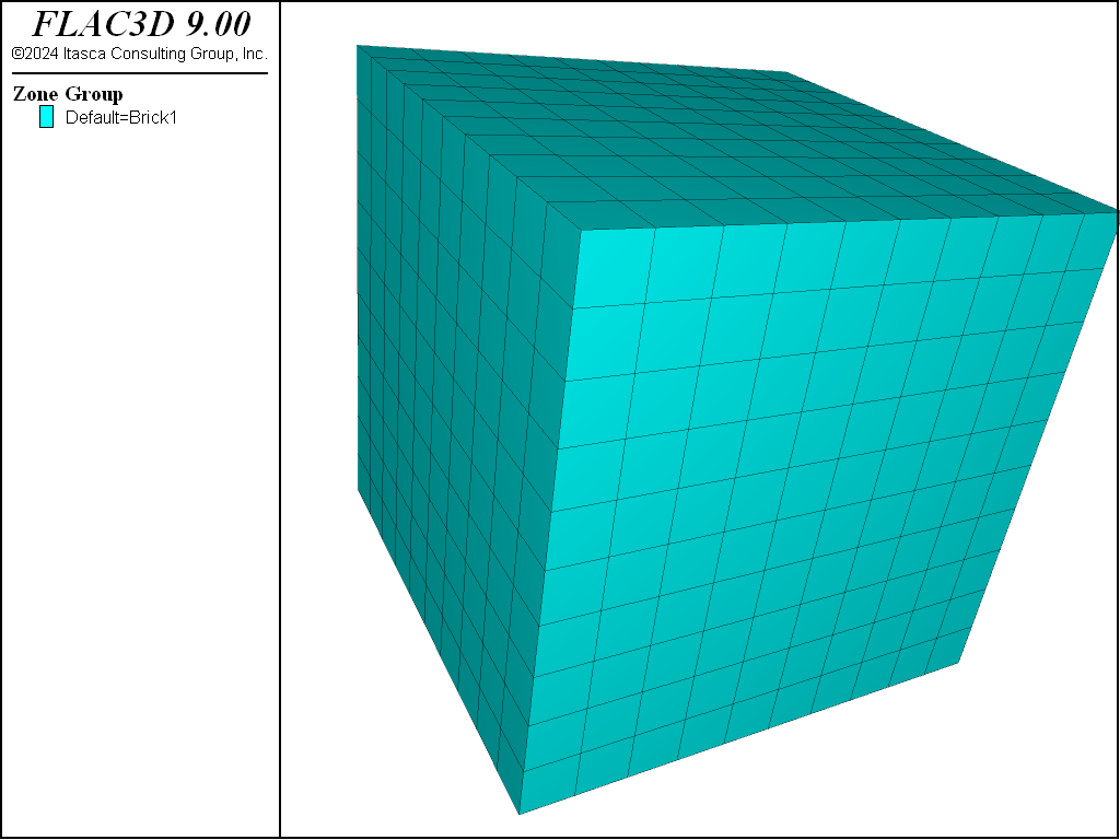
Figure 1: Finite volume grid with 1000 zones.
Nomenclature
FLAC3D uses nomenclature that is consistent, in general, with that used in conventional finite volume or finite element programs for stress analysis. The basic definitions of terms are reviewed here for clarification. The figure below illustrates the FLAC3D terminology.
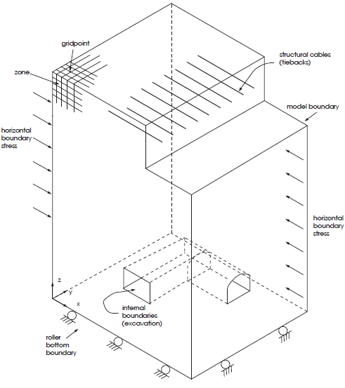
Figure 2: Example of a FLAC3D model.
Endnotes
| Was this helpful? ... | Itasca Software © 2024, Itasca | Updated: Nov 12, 2025 |
