FLAC3D Theory and Background • Fluid-Mechanical Interaction

One-Dimensional Filling of a Porous Region

Note

To view this project in FLAC3D, use the menu command Help ► Examples…. The project’s main data files are shown at the end of this example.

In this problem, flow is driven through an initially dry porous layer of large lateral extent under a constant pressure, \(p_{_{o}}\), applied at the base. The transient location of the filling front is compared to an exact sharp-front solution for the cases with and without gravity.

Voller et al. (1996) give an analytic solution for this problem under the assumptions of a sharp-front, rigid-porous matrix and incompressible Newtonian fluid. In their solution, the flow is governed by Darcy’s law, and there is a constant atmospheric pressure in the air ahead of the free surface.

Let the \(x\)-axis of reference be oriented in the direction of flow, with the origin at the base of the layer. The solution for the front location, \(x_{f}\), may be expressed in terms of two dimensionless variables: \(\widehat{t}=\) \(t/T^{\ast }\)and \(\widehat{x}=x_{f}/L^{\ast }\); and a dimensionless parameter, \(\gamma\), defined using the expressions \(T^{\ast}=n\mu /p_{o}\), \(\ L^{\ast }=\sqrt{\kappa }\) and \(\gamma =\sqrt{\kappa }\) \(\rho g/p_{o}\). In these equations, \(n\) is porosity, \(\kappa\) is intrinsic permeability (product of mobility coefficient, \(k\), and dynamic viscosity, \(\mu\)), \(\rho\) is fluid density, and \(g\) is gravity.

When gravity is ignored, the solution has the form

(1)\[\widehat{t}={{1}\over{2}} \left[ \widehat{x} \right] ^{2}\]

For filling under gravity, the front location is given by

(2)\[\widehat{t}=-{\widehat{x}\over\gamma} -{\ln \left( 1-\gamma \widehat{x}\right) \over\gamma ^{2}}\]

Equation (2) may be shown to converge to the no-gravity solution when \(\gamma\) goes to zero.

The numerical solution to the filling problem is presented in dimensionless form. To derive this solution, scaled properties are used in the simulations: \(p_{o}\) = 1, \(k\) = 0.25, \(n\) = 0.5; and for gravity flow, \(\rho _{w}\) = 1 and \(g\) = 1. Further, using \(\mu\) = 4 in the preceding definitions, the characteristic parameters for the simulation are \(T^{\ast }\) = 2, \(L^{\ast }\) = 1, \(\gamma\) = 1.

To simulate incompressible flow, the bulk modulus of the fluid, \(K_{f}\), is assigned a value that is large compared to the pore-pressure variations in the simulation (\(K_{f}\) = 100). For both cases, the grid corresponds to a column of 25 zones, 0.625 units high and 0.025 units wide. The initial value of pore pressure and saturation is zero. The pore pressure is fixed at \(p_{o}\), and the saturation is given a value of 1 at the base of the model. The simulation is conducted for a total of 0.25 units of time (\(\widehat{t}\) = 0.125). A FISH function, flacfront, captures the times at which nodes reach a saturation of 1% and 99%. The analytic sharp-front solution is evaluated by another FISH function, solution. The data file for the case without gravity is listed in “1DFillingPorousRegion-NoGravity.dat”; the data file for the case with gravity is listed in “1DFillingPorousRegion-Gravity.dat”.

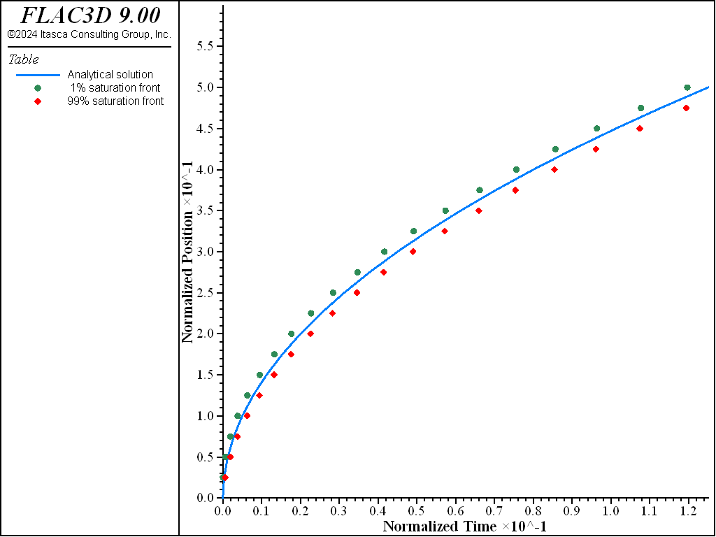
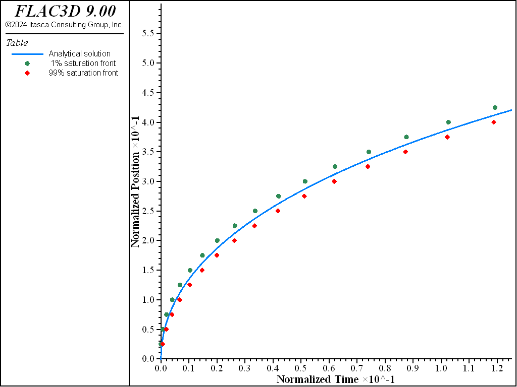
The results with and without gravity are presented in Figure 1 and Figure 2, respectively. As seen in these figures, the sharp-front solution is bounded above and below by the 99% and 1% saturation fronts. In fact, the vertical distance between these fronts corresponds directly to the grid size in the direction of propagation of the filling front. (The saturation at a node can only start to increase when the pore pressure at the node below it becomes positive, and thus full saturation is reached there.) This distance can be reduced by increasing the number of zones in the column height. The evolution of nodal pore pressure with time follows a stepwise pattern, more pronounced as the fluid is less compressible. This behavior occurs because a node must be fully saturated before its pore pressure can increase. One way to reduce this effect without changing the grid size is to introduce flow in the unsaturated region (capillary pressure) in the fluid flow formulation.

break

Figure 1: Location of filling front (\(\widehat{x}\) vs \(\widehat{t}\)) — no gravity (analytical solution = solid line; numerical values = dotted lines).

Figure 2: Location of filling front (\(\widehat{x}\) vs \(\widehat{t}\)) — with gravity (analytical solution = solid line; numerical values = dotted lines).

Data Files

1DFillingPorousRegion-NoGravity.dat

model new
model large-strain off
model title "One-dimensional filling - no gravity"
fish automatic-create off
model configure fluid
program call 'fishFunctions'
[setup]
zone create brick size 1 1 25 point 1 (0.025,0,0) point 2 (0,0.025,0) ...
                              point 3 (0,0,0.625)
; --- fluid flow model ---
zone fluid cmodel assign isotropic
zone fluid property permeability [c_perm] porosity [c_poro] biot 0. ; 
zone fluid biot on
zone gridpoint initialize biot 100
zone gridpoint initialize saturation 0.0
zone face apply pore-pressure [c_p0] range position-z 0
; --- settings ---
model mechanical active off
model fluid active on
[solution1]
table '1' label 'Analytical solution'
table '2' label ' 1% saturation front'
table '3' label '99% saturation front'
; --- test ---
[global lzf=0.025, uzf=0.025]
model solve fluid time-total 0.25
model save 'asat1'
program return

1DFillingPorousRegion-Gravity.dat

model new
model large-strain off
model title "One-dimensional filling - with gravity"
fish automatic-create off
model configure fluid
program call 'fishFunctions'
[setup]
zone create brick size 1 1 25 point 1 (0.025,0,0) point 2 (0,0.025,0) ...
                              point 3 (0,0,0.625)
; --- fluid flow model ---
zone fluid cmodel assign isotropic
zone fluid property permeability [c_perm] porosity [c_poro] biot 0. 
zone fluid biot on
zone gridpoint initialize biot 100
zone gridpoint initialize saturation 0.0
zone face apply pore-pressure [c_p0] range position-z 0
; --- settings ---
zone initialize fluid-density [c_den]
model gravity 0 0 [c_grav]
model mechanical active off
model fluid active on
[solution2]
table '1' label 'Analytical solution'
table '2' label ' 1% saturation front'
table '3' label '99% saturation front'
; --- test ---
[global lzf=0.025, uzf=0.025]
model solve fluid time-total 0.25
model save 'asat2'
program return