0.0 - Timestep Determination

Overview

In order to reliably update the model state, one must determine a suitable timestep for the numerical integration of Newton’s laws. Selection of a timestep that is too large may result in instability manifested by bodies flying off to infinity. On the other hand, selection of a timestep that is too small may result in excessively long simulation times. In PFC, the timestep is calculated based on kinematic constraints on piece displacement and stiffness constraints as outlined below; the final timestep is taken as the minimum of these constraints. Timestep computations may be relatively expensive and one may, with great caution, disable the timestep calculation algorithm altogether to improve efficiency. This is a dangerous proposition and should only be used by advanced users.

Detailed Description

The model mechanical timestep command can be used to specify if the timestep will be fixed, if timestep scaling will be active or if the timestep will be determined automatically. Each of these scenarios are discussed below in detail. Before embarking on these topics, the kinematic timestep constraints are discussed. These correspond with piece displacement constraints and are used to ensure that contacts are created prior to the development of forces/moments.

Note that, as described in this section, the Velocity Verlet algorithm is used to integrate Newton’s laws. In terms of when they are updated, the velocities are 1/2 a timestep out of phase compared with the body positions. At the beginning of this cycle point, the velocities of balls and clumps are updated as described in that section.

Kinematic Timestep Constraints

Whether using the timestep scaling or automatic timestep determination mode, PFC imposes a kinematic constraint on the timestep in order to guarantee that contacts are created between pieces prior to the cycle that forces/moments develop. This constraint is described in detail here. From that discussion, the kinematic constraint that a piece may only translate \(\varepsilon\) during any cycle is imposed to ensure proper contact creation. To enforce this displacement constraint, the timestep is limited as follows.

Using Newton’s second law, one can calculate a component of the translational acceleration as

(1)\[a_i = \frac{(F_i + g_i * m_g + Fa_i)}{m_i}\]

where \(F_i\) is the contact force, \(g_i\) is the force of gravity, \(m_g\) is the gravitational mass, \(Fa_i\) is the applied force, and \(m_i\) is the inertial mass. The subscript \(i\) refers to the ith component component of these vectors. Take \(a_{\rm max}\) to be the maximum absolute translational acceleration taken over all components.

The expression for the displacement of a rigid body acted upon by a constant acceleration for a time of duration \(t\) is given by

(2)\[x = v_0 * t + 1/2 * a * t^2\]

where \(x\) is the displacement, \(v_0\) is the initial velocity and \(a\) is the constant acceleration acting during time \(t\). This expression can be rearranged to calculate the time required for a rigid body experiencing constant acceleration to translate a specified amount

(3)\[t = \frac{(- v_0 + \sqrt{{v_0}^2 + 2 * a * x})}{a}\]

Suppose that the maximum absolute component of the piece translational velocity is given by \(v_{\rm max}\). For balls, this is the translational velocity at its centroid. For pebbles (facets), this corresponds to the translational clump (wall) velocity plus the translational velocity due to the clump (wall) rotation at the pebble centroid (facet periphery). The kinematic timestep constraint is the duration of time for the piece to translate \(\varepsilon\), or

(4)\[t_{\rm kin} = \frac{(- v_{\rm max} + \sqrt{{v_{\rm max}}^2 + 2 * a_{\rm max} * \varepsilon})} {a_{\rm max}}\]

Fixed Timestep

All operations that occur during this cycle point are skipped when the timestep is fixed to a user-specified value. There are many computations that occur if the automatic timestep determination mode is active and one can gain a fair degree of performance by fixing the timestep. On the other hand, model instability may result. For instance, pieces may fly through one another in a single cycle without any forces developing. Additionally, large overlaps can occur in a single cycle resulting in large forces. This can cause a nearly static assembly to blow apart in an unphysical fashion. It is the user’s responsibility to ensure stability when this mode is activated.

Timestep Scaling

The default behavior of PFC is to automatically determine the critical timestep using the procedure outlined in the next section. This provides a true dynamic solution that is valid for both steady-state and non-steady-state conditions. If one is interested only in obtaining the steady-state solution (in which all particle acceleration is zero, corresponding to either a static equilibrium or a steady flow), timestep scaling may be used as a means to reach the steady state configuration with as few computational cycles as possible. The path to this final configuration is unphysical in the sense that the masses and velocities have been scaled to achieve rapid convergence. Body forces, such as gravitational forces, are not affected when timestep scaling is active. The scaling operations described below occur during this cycle point.

Because the stable timestep is proportional to the square root of the mass of a body divided by the sum of the stiffnesses acting on the body (see Equation (11)), a few small particles (or ones with high stiffnesses) may cause the timestep to be very small. When timestep scaling is active, a fictitious inertial mass is calculated for each body such that its stable timestep is 1 by default. The user may specify a value different from 1 if desired. The body’s velocity must also be scaled proportionally to ensure stability.

Suppose that the timestep is set to \(\Delta t\). The new inertial mass of a body is calculated by

(5)\[m_{\rm new} = k^{\rm tran} * {\Delta t}^2\]

where \(m_i\) is the body’s inertial mass and \(k^{\rm tran}\) is the maximum component of the total translational stiffness acting on the body. The velocity vector of the body is scaled, as well

(6)\[{\mathbf v}_{\rm new} = {\mathbf v} * m_i / m_{\rm new}\]

Likewise, a scaled moment of inertia is calculated by

(7)\[{\mathbf{I}}_{\rm new} = k^{\rm rot} * {\Delta t}^2\]

where \({\mathbf{I}}_i\) is the body’s unscaled moment of inertia and \(k^{\rm rot}\) is the maximum component of the total angular stiffness acting on the body. The angular velocity vector of the body is scaled proportionally

(8)\[\pmb{\omega}_{\rm new} = \pmb{\omega} * {\mathbf{I}}_i / {\mathbf{I}}_{new}\]

These scaling operations result in all degrees of freedom in the system having equal time responses, meaning that the assembly converges to a static state more rapidly. As a consequence, the timescale is meaningless. Timestep scaling should only be used if there are large differences in particle sizes and/or there are large stiffness differences present and a rapid convergence to static equilibrium is required. The scaling should not be used if the solution is path-dependent, because the path followed, although valid, is unphysical. It is important to remember that there are an infinite number of possible solutions to a nonlinear, inelastic problem, depending on path. The timestep scaling mode corresponds to the differential density scaling mode in previous versions of PFC.

Automatic Timestep Determination

In order for the explicit solution of Newton’s laws to remain stable, the timestep must not exceed a critical value that is related to the minimum eigen-period of the total system. However, global eigenvalue analyses are impractical to apply to the large and constantly changing systems typically encountered in PFC simulations. Therefore, a simplified procedure is implemented to estimate the critical timestep. The actual timestep used in any cycle is taken as a fraction of this estimated critical value (see the model mechanical timestep safety-factor command).

Estimation Procedure for Solution Stability

First, consider a one-dimensional mass-spring system described by a point mass \(m\), and spring with stiffness \(k\), with the coordinate system shown in Figure 1. The motion of the point mass is governed by the differential equation \(-kx = m \ddot x\). The critical timestep corresponding to a second-order finite-difference scheme for this equation is given by Bathe and Wilson ([Bathe1976]):

(9)\[t_{\rm{crit}} = {T \over \pi}; \qquad T = 2 \pi \sqrt{m/k}\]

where \(T\) is the period of the system.

Next, consider the infinite series of point masses and springs in Figure 2. The smallest period of this system will occur when the masses are moving in synchronized opposing motion such that there is no motion at the center of each spring. The motion of a single point mass can be described by the two equivalent systems shown in that figure. Using Equation (9), the critical timestep for this system is found to be

(10)\[t_{\rm crit} = 2\sqrt{m/(4k)} = \sqrt{m/k}\]

where \(k\) is the stiffness of each of the springs in Figure 2.

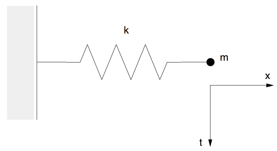
Figure 1: Single mass-spring system.

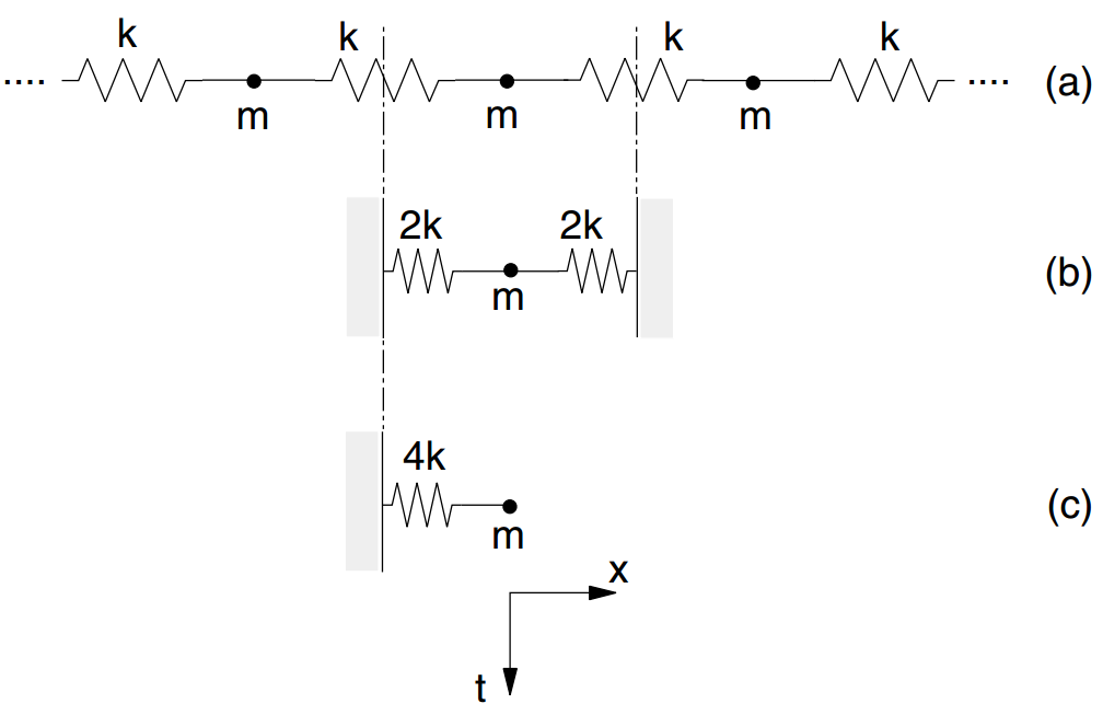
Figure 2: Multiple mass-spring system.

These two systems characterize translational motion. Rotational motion is characterized by the same two systems in which mass \(m\), is replaced by moment of inertia \(I\), of a finite-sized particle, and the stiffness is replaced by the rotational stiffness. Thus, the critical timestep for the generalized multiple mass-spring system can be expressed as

(11)\[\begin{split}t_{\rm crit} = \begin{cases} \sqrt{m/k^{\rm tran}}, &\mbox{(translational motion)} \\ \sqrt{I/k^{\rm rot}}, &\mbox{(rotational motion)} \end{cases}\\\end{split}\]

where \(k^{\rm tran}\) and \(k^{\rm rot}\) are the translational and rotational stiffnesses, respectively, and \(I\) is the moment of inertia of the particle.

The model components in PFC are conceptualized as a collection of discrete bodies composed of {disk shaped balls/pebbles in 2D; spherical balls/pebbles in 3D} and springs. Each body may have a different mass, and each spring may have a different stiffness. A critical timestep is found for each body by applying Equation (11) separately to each degree of freedom, assuming that the degrees of freedom are uncoupled. The stiffnesses are estimated by summing the contribution from all contacts using only the diagonal terms of the contact stiffness matrix. The final critical timestep is taken to be the minimum of all critical timesteps computed for all degrees of freedom of all bodies.

Contact Stiffness Matrix

The stiffness matrix at a contact between two pebbles is given here (see [Potyondy2009] for the full derivation). First, the 3D relations are described. Then the simplified 2D relations are also presented.

Each contact exists between two discrete pieces, each of which has six degrees of freedom at its center of mass of the body in 3D. If we refer to the centers of mass as nodes, then we can say that each contact has a stiffness matrix that relates generalized forces and displacements at the two nodes that it joins. The nodal degrees of freedom contain three translational components and three rotational components. The generalized displacements and forces at node \(i\) are denoted by

(12)\[\begin{split}\{{\bf d_i}\} &= \lfloor u_i \ v_i \ w_i \ \theta_{xi} \ \theta_{yi} \ \theta_{zi} \rfloor^T \\ \{{\bf r_i}\} &= \lfloor F_{xi} \ F_{yi} \ F_{zi} \ M_{xi} \ M_{yi} \ M_{zi} \rfloor^T\end{split}\]

and shown in the figure below:

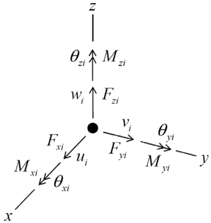
Figure 3: Generalized displacements and forces at node \(i\).

The 3D stiffness matrix of a contact joining nodes \(a\) and \(b\) relates the generalized forces to the generalized displacements via

(13)\[\begin{split}\left\{\begin{matrix} {\bf r_a} \\ {\bf r_b} \end{matrix}\right\} = {\bf [k]} \left\{\begin{matrix} {\bf d_a} \\ {\bf d_b} \end{matrix}\right\} \Longleftrightarrow \left\{\begin{matrix} F_{xa} \\ F_{ya} \\ F_{za} \\ M_{xa} \\ M_{ya} \\ M_{za} \\ F_{xb} \\ F_{yb} \\ F_{zb} \\ M_{xb} \\ M_{yb} \\ M_{zb} \end{matrix}\right\} = {\bf [k]} \left\{\begin{matrix} u_a \\ v_a \\ w_a \\ \theta_{xa} \\ \theta_{ya} \\ \theta_{za} \\ u_b \\ v_b \\ w_b \\ \theta_{xb} \\ \theta_{yb} \\ \theta_{zb} \end{matrix}\right\}\end{split}\]

A typical contact joining two pebbles of separate clumps is shown in Figure 4. The system is defined by the centers of mass of clumps \(a\) and \(b\) (\(\bf x_a\) and \(\bf x_b\), respectively), the contact location (\(\bf x_c\)), a unit-vector triad (\(\bf n1\), \(\bf n2\) and \(\bf n3\)) such that \(\bf n_3\) is aligned with the contact-normal direction, and the contact translational (\(k_n\) and \(k_s\)) and rotational (\(k_{n \theta}\) and \(k_{s \theta}\)) stiffnesses. We also define \(\bf R_a = x_c - x_a\) and \(\bf R_b = x_c - x_b\).

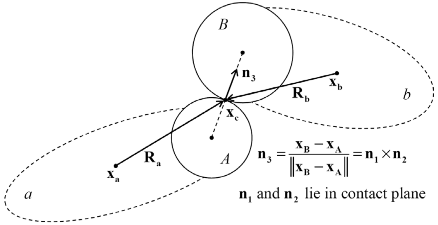
Figure 4: Typical DEM contact between two pebbles.

The 3D stiffness matrix is symmetric. Thus, it can be expressed as

(14)\[\begin{split} {\bf [k]} = \left[\begin{matrix} k_{1,1} & {} & {} & {} & {} & {} & {} & {} & {} & {} \\ k_{2,1} & k_{2,2} & {} & {} & {} & {} & {} & {} & {} & {} \\ \vdots & {} &\ddots & {} & {} & {} & {} & {} & {} & {} \\ {} & {} & {} & {} & {} & {\rm symmetric} & {} & {} & {} & {} \\ {} & {} & {} & {} & {} & {} & {} & {} & {} & {} \\ {} & {} & {} & {} & {} & {} & {} & {} & {} & {} \\ {} & {} & {} & {} & {} & {} & {} & {} & {} & {} \\ {} & {} & {} & {} & {} & {} & {} & {} & {} & {} \\ {} & {} & {} & {} & {} & {} & {} & {} & {} & {} \\ {} & {} & {} & {} & {} & {} & {} & \ddots & {} & {} \\ \vdots & {} & {} & {} & {} & {} & {} & {} & k_{11,11} & {} \\ k_{12,1} & \cdots & {} & {} & {} & {} & {} & \cdots & k_{12,11} & k_{12,12} \end{matrix}\right]\end{split}\]

The individual terms are expressed in the global coordinate system in terms of the DEM contact quantities in 3D and are listed as follows, with each group designating the lower-diagonal portion of a set of columns. For columns 1 to 3:

(15)\[\begin{split}k_{1,1} &= k_s (n_{x1} n_{x1} + n_{x2} n_{x2}) + k_n n_{x3} n_{x3} \qquad k_{7,1} = - k_{1,1} \\ k_{2,1} &= k_s (n_{y1} n_{x1} + n_{y2} n_{x2}) + k_n n_{y3} n_{x3} \qquad k_{8,1} = - k_{2,1} \\ k_{3,1} &= k_s (n_{z1} n_{x1} + n_{z2} n_{x2}) + k_n n_{z3} n_{x3} \qquad k_{9,1} = - k_{3,1} \\ k_{4,1} &= R_{ya} k_{3,1} - R_{za} k_{2,1} \ \ \ \ \ \ \ \ \ \ \ \ \ \ \ \ \ \qquad k_{10,1} = -R_{yb} k_{3,1} + R_{zb} k_{2,1} \\ k_{5,1} &= R_{za} k_{1,1} - R_{xa} k_{3,1} \ \ \ \ \ \ \ \ \ \ \ \ \ \ \ \ \ \qquad k_{11,1} = -R_{zb} k_{1,1} + R_{xb} k_{3,1} \\ k_{6,1} &= R_{xa} k_{2,1} - R_{ya} k_{1,1} \ \ \ \ \ \ \ \ \ \ \ \ \ \ \ \ \ \qquad k_{12,1} = -R_{xb} k_{2,1} + R_{yb} k_{1,1}\end{split}\]

(16)\[\begin{split}{} k_{7,2} &= - k_{1,2} \\ k_{2,2} = k_s (n_{y1} n_{y1} + n_{y2} n_{y2}) + k_n n_{y3} n_{y3} \ \ \ k_{8,2} &= - k_{2,2} \\ k_{3,2} = k_s (n_{z1} n_{y1} + n_{z2} n_{y2}) + k_n n_{z3} n_{y3} \ \ \ k_{9,2} &= - k_{3,2} \\ k_{4,2} = R_{ya} k_{3,2} - R_{za} k_{2,2} \ \ \ \ \ \ \ \ \ \ \ \ k_{10,2} &= -R_{yb} k_{3,2} + R_{zb} k_{2,2} \\ k_{5,2} = R_{za} k_{1,2} - R_{xa} k_{3,2} \ \ \ \ \ \ \ \ \ \ \ \ \ \ \ k_{11,2} &= -R_{zb} k_{1,2} + R_{xb} k_{3,2} \\ k_{6,2} = R_{xa} k_{2,2} - R_{ya} k_{1,2} \ \ \ \ \ \ \ \ \ \ \ \ \ \ \ k_{12,2} &= -R_{xb} k_{2,2} + R_{yb} k_{1,2}\end{split}\]

(17)\[\begin{split}{} \ \ \ \ \ \ \ \ \ \ \ \ \ \ \ \ \ \ \ \ \ \ \ \ \ \ \ \ \ \ \ \ \ \ \ k_{7,3} &= - k_{1,3} \\ {} \ \ \ \ \ \ \ \ \ \ \ \ \ \ \ \ \ \ \ \ \ \ \ \ \ \ \ \ \ \ \ \ \ \ \ k_{8,3} &= - k_{2,3} \\ k_{3,3} = k_s (n_{z1} n_{z1} + n_{z2} n_{z2}) + k_n n_{z3} n_{z3} \ \ \ \ k_{9,3} &= - k_{3,3} \\ k_{4,3} = R_{ya} k_{3,3} - R_{za} k_{2,3} \ \ \ \ \ \ \ \ \ \ \ \ \ \ \ \ k_{10,3} &= -R_{yb} k_{3,3} + R_{zb} k_{2,3} \\ k_{5,3} = R_{za} k_{1,3} - R_{xa} k_{3,3} \ \ \ \ \ \ \ \ \ \ \ \ \ \ \ \ k_{11,3} &= -R_{zb} k_{1,3} + R_{xb} k_{3,3} \\ k_{6,3} = R_{xa} k_{2,3} - R_{ya} k_{1,3} \ \ \ \ \ \ \ \ \ \ \ \ \ \ \ k_{12,3} &= -R_{xb} k_{2,3} + R_{yb} k_{1,3}\end{split}\]

For columns 4 to 6:

(18)\[\begin{split}k_{4,4} &= k_{s \theta} (n_{x1} n_{x1} + n_{x2} n_{x2}) + k_{n \theta} n_{x3} n_{x3} + (R_{ya} k_{3,4} - R_{za} k_{2,4}) \\ k_{5,4} &= k_{s \theta} (n_{y1} n_{x1} + n_{y2} n_{x2}) + k_{n \theta} n_{y3} n_{x3} + (R_{za} k_{1,4} - R_{xa} k_{3,4}) \\ k_{6,4} &= k_{s \theta} (n_{z1} n_{x1} + n_{z2} n_{x2}) + k_{n \theta} n_{z3} n_{x3} + (R_{xa} k_{2,4} - R_{ya} k_{1,4}) \\ k_{7,4} &= -k_{1,4} \\ k_{8,4} &= -k_{2,4} \\ k_{9,4} &= -k_{3,4} \\ k_{10,4} &= -k_{s \theta} (n_{x1} n_{x1} + n_{x2} n_{x2}) - k_{n \theta} n_{x3} n_{x3} + (-R_{yb} k_{3,4} + R_{zb} k_{2,4}) \\ k_{11,4} &= -k_{s \theta} (n_{y1} n_{x1} + n_{y2} n_{x2}) - k_{n \theta} n_{y3} n_{x3} + (-R_{zb} k_{1,4} + R_{xb} k_{3,4}) \\ k_{12,4} &= -k_{s \theta} (n_{z1} n_{x1} + n_{z2} n_{x2}) - k_{n \theta} n_{z3} n_{x3} + (-R_{xb} k_{2,4} + R_{yb} k_{1,4})\end{split}\]

(19)\[\begin{split}k_{5,5} &= k_{s \theta} (n_{y1} n_{y1} + n_{y2} n_{y2}) + k_{n \theta} n_{y3} n_{y3} + (R_{za} k_{1,5} - R_{xa} k_{3,5}) \\ k_{6,5} &= k_{s \theta} (n_{z1} n_{y1} + n_{z2} n_{y2}) + k_{n \theta} n_{z3} n_{y3} + (R_{xa} k_{2,5} - R_{ya} k_{1,5}) \\ k_{7,5} &= -k_{1,5} \\ k_{8,5} &= -k_{2,5} \\ k_{9,5} &= -k_{3,5} \\ k_{10,5} &= -k_{s \theta} (n_{x1} n_{y1} + n_{x2} n_{y2}) - k_{n \theta} n_{x3} n_{y3} + (-R_{yb} k_{3,5} + R_{zb} k_{2,5}) \\ k_{11,5} &= -k_{s \theta} (n_{y1} n_{y1} + n_{y2} n_{y2}) - k_{n \theta} n_{y3} n_{y3} + (-R_{zb} k_{1,5} + R_{xb} k_{3,5}) \\ k_{12,5} &= -k_{s \theta} (n_{z1} n_{y1} + n_{z2} n_{y2}) - k_{n \theta} n_{z3} n_{y3} + (-R_{xb} k_{2,5} + R_{yb} k_{1,5})\end{split}\]

(20)\[\begin{split}k_{6,6} &= k_{s \theta} (n_{z1} n_{z1} + n_{z2} n_{z2}) + k_{n \theta} n_{z3} n_{z3} + (R_{xa} k_{2,6} - R_{ya} k_{1,6}) \\ k_{7,6} &= -k_{1,6} \\ k_{8,6} &= -k_{2,6} \\ k_{9,6} &= -k_{3,6} \\ k_{10,6} &= -k_{s \theta} (n_{x1} n_{z1} + n_{x2} n_{z2}) - k_{n \theta} n_{x3} n_{z3} + (-R_{yb} k_{3,6} + R_{zb} k_{2,6}) \\ k_{11,6} &= -k_{s \theta} (n_{y1} n_{z1} + n_{y2} n_{z2}) - k_{n \theta} n_{y3} n_{z3} + (-R_{zb} k_{1,6} + R_{xb} k_{3,6}) \\ k_{12,6} &= -k_{s \theta} (n_{z1} n_{z1} + n_{z2} n_{z2}) - k_{n \theta} n_{z3} n_{z3} + (-R_{xb} k_{2,6} + R_{yb} k_{1,6})\end{split}\]

For columns 7 to 9:

(21)\[\begin{split}k_{7,7} &= k_{1,1} \\ k_{8,7} &= k_{2,1} \\ k_{9,7} &= k_{3,1} \\ k_{10,7} &= -R_{yb} k_{3,7} + R_{zb} k_{2,7} \\ k_{11,7} &= -R_{zb} k_{1,7} + R_{xb} k_{3,7} \\ k_{12,7} &= -R_{xb} k_{2,7} + R_{yb} k_{1,7} \\ k_{8,8} &= k_{2,2} \\ k_{9,8} &= k_{3,2} \\ k_{10,8} &= -R_{yb} k_{3,8} + R_{zb} k_{2,8} \\ k_{11,8} &= -R_{zb} k_{1,8} + R_{xb} k_{3,8} \\ k_{12,8} &= -R_{xb} k_{2,8} + R_{yb} k_{1,8} \\ k_{9,9} &= k_{3,3} \\ k_{10,9} &= -R_{yb} k_{3,9} + R_{zb} k_{2,9} \\ k_{11,9} &= -R_{zb} k_{1,9} + R_{xb} k_{3,9} \\ k_{12,9} &= -R_{xb} k_{2,9} + R_{yb} k_{1,9}\end{split}\]

For columns 10 to 12:

(22)\[\begin{split}k_{10,10} &= k_{s \theta} (n_{x1} n_{x1} + n_{x2} n_{x2}) + k_{n \theta} n_{x3} n_{x3} + (-R_{yb} k_{3,10} + R_{zb} k_{2,10}) \\ k_{11,10} &= k_{s \theta} (n_{y1} n_{x1} + n_{y2} n_{x2}) + k_{n \theta} n_{y3} n_{x3} + (-R_{zb} k_{1,10} + R_{xb} k_{3,10}) \\ k_{12,10} &= k_{s \theta} (n_{z1} n_{x1} + n_{z2} n_{x2}) + k_{n \theta} n_{z3} n_{x3} + (-R_{xb} k_{2,10} + R_{yb} k_{1,10}) \\ k_{11,11} &= k_{s \theta} (n_{y1} n_{y1} + n_{y2} n_{y2}) + k_{n \theta} n_{y3} n_{y3} + (-R_{zb} k_{1,11} + R_{xb} k_{3,11}) \\ k_{12,11} &= k_{s \theta} (n_{z1} n_{y1} + n_{z2} n_{y2}) + k_{n \theta} n_{z3} n_{y3} + (-R_{xb} k_{2,11} + R_{yb} k_{1,11}) \\ k_{12,12} &= k_{s \theta} (n_{z1} n_{z1} + n_{z2} n_{z2}) + k_{n \theta} n_{z3} n_{z3} + (-R_{xb} k_{2,12} + R_{yb} k_{1,12})\end{split}\]

In 2D, the stiffness matrix is obtained from the 3D equivalent. The 2D model has 3 degrees of freedom per node, therefore \(\omega= \theta_x = \theta_y \equiv 0\) and the 2D stiffness matrix is reduced to

(23)\[\begin{split}\left\{\begin{matrix} {\bf r_a} \\ {\bf r_b} \end{matrix}\right\} = {\bf [k]} \left\{\begin{matrix} {\bf d_a} \\ {\bf d_b} \end{matrix}\right\} \Longleftrightarrow \left\{\begin{matrix} F_{xa} \\ F_{ya} \\ M_{za} \\ F_{xb} \\ F_{yb} \\ M_{zb} \end{matrix}\right\} = {\bf [k]} \left\{\begin{matrix} u_a \\ v_a \\ \theta_{za} \\ u_b \\ v_b \\ \theta_{zb} \end{matrix}\right\}\end{split}\]

We align the unit-vector triad such that \(\bf{n_1}\) and \(\bf{n_3}\) lie in the global xy-plane, and choose \(\bf{n_1}\) such that \(\bf{n_3} \times \bf{n_1} = + \bf{\hat{j}} = \bf{n_2}\). The system is shown in the figure below and has the form

(24)\[\begin{split}\bf{n_3} = \left\{\begin{matrix} {n_{x3}} \\ {n_{y3}} \\ {0} \end{matrix}\right\} , \bf{n_1} = \left\{\begin{matrix} {n_{x1}} \\ {n_{y1}} \\ {0} \end{matrix}\right\} = \left\{\begin{matrix} {-n_{y3}} \\ {n_{x3}} \\ {0} \end{matrix}\right\} , \bf{n_2} = \left\{\begin{matrix} {0} \\ {0} \\ {1} \end{matrix}\right\}\end{split}\]

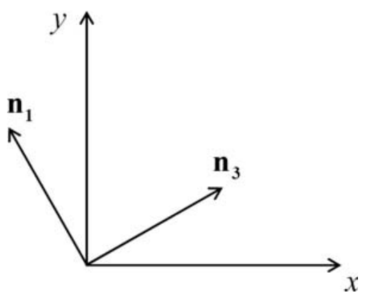
Figure 5: Orientation of unit-vector triad in 2D model.

The resulting 2D stiffness matrix relating the degrees of freedom in Equation (23) can be expressed as

(25)\[\begin{split} {\bf [k]} = \left[\begin{matrix} k_{1,1} & {} & {} & {} & {} & {} \\ k_{2,1} & k_{2,2} & {} & sym. & {} & {} \\ \vdots & {} &\ddots & {} & {} & {} \\ {} & {} & {} &\ddots & {} & {} \\ \vdots & {} & {} & {} & k_{5,5} & {} \\ k_{6,1} & \cdots & {} & \cdots & k_{6,5} & k_{6,6} \end{matrix}\right]\end{split}\]

The individual terms are expressed in the global coordinate system in terms of the DEM contact quantities and are listed as follows, with each group designating the lower-diagonal portion of a set of columns. For the first two columns:

(26)\[\begin{split}k_{1,1} &= k_s (n_{x1} n_{x1} + k_n n_{x3} n_{x3} = k_s {n_{y3}}^2 + k_n {n_{x3}}^2 \\ k_{2,1} &= k_s (n_{y1} n_{x1} + k_n n_{y3} n_{x3} \\ k_{3,1} &= R_{xa} k_{2,1} - R_{ya} k_{1,1} \\ k_{4,1} &= - k_{1,1} \\ k_{5,1} &= - k_{2,1} \\ k_{6,1} &= R_{xb} k_{2,1} + R_{yb} k_{1,1} \\ k_{2,2} &= k_s (n_{y1} n_{y1} + k_n n_{y3} n_{y3} = k_s {n_{x3}}^2 + k_n {n_{y3}}^2 \\ k_{3,2} &= R_{xa} k_{2,2} - R_{ya} k_{1,2} \\ k_{4,2} &= - k_{1,2} \\ k_{5,2} &= - k_{2,2} \\ k_{6,2} &= -R_{xb} k_{2,2} + R_{yb} k_{1,2}\end{split}\]

For the last four columns:

(27)\[\begin{split}k_{3,3} &= k_{s\theta} + (R_{xa} k_{2,3} - R_{ya} k_{1,3}) \\ k_{4,3} &= - k_{1,3} \\ k_{5,3} &= - k_{2,3} \\ k_{6,3} &= -k_{s\theta} + (-R_{xb} k_{2,3} + R_{yb} k_{1,3}) \\ k_{4,4} &= k_{1,1} \\ k_{5,4} &= k_{2,1} \\ k_{6,4} &= -R_{xb} k_{2,4} + R_{yb} k_{1,4} \\ k_{5,5} &= k_{2,2} \\ k_{6,5} &= -R_{xb} k_{2,5} + R_{yb} k_{1,5} \\ k_{6,6} &= k_{s\theta} + (-R_{xb} k_{2,6} + R_{yb} k_{1,6})\end{split}\]

– Next Cycle Point: Law of Motion –

References

[Bathe1976]

Bathe, K. J., and E. L. Wilson. Numerical Methods in Finite Element Analysis. Englewood Cliffs: Prentice-Hall, 1976.

[Potyondy2009]

Potyondy, D. “Stiffness Matrix at a Contact Between Two Clumps,” Itasca Consulting Group, Inc., Minneapolis, MN, Technical Memorandum ICG6863-L, December 7,2009.