Zones

Overview of Constitutive Models

This section provides an overview of the constitutive models in 3DEC and makes recommendations concerning their appropriate application. The Constitutive Models section presents background information on the model formulations.

The built-in zone mechanical material models [1] in 3DEC are shown in the following table:

Table 1: 3DEC Zone Constitutive Models

Model	Representative Material	Example Application
(Isotropic) elastic	homogeneous, isotropic continuum; linear stress-strain behavior	manufactured materials (e.g., steel) loaded below strength limit; factor of safety calculation
Orthotropic elastic	materials with three mutually perpendicular planes of elastic symmetry	columnar basalt loaded below strength limit
Anisotropic (transversely isotropic) elastic	thinly laminated material exhibiting elastic anisotropy (e.g., slate)	laminated materials loaded below strength limit
Drucker-Prager	limited application; soft clays with low friction	common model for comparison to implicit finite-element programs
Mohr-Coulomb	loose and cemented granular materials; soils, rock, concrete	general soil or rock mechanics (e.g., slope stability and underground excavation)
Strain-hardening/softening Mohr-Coulomb	granular materials that exhibit nonlinear material hardening or softening	studies in post-failure (e.g., progressive collapse, yielding pillar, caving)
Ubiquitous-joint	thinly laminated material exhibiting strength anisotropy (e.g., slate)	excavation in closely bedded strata
Anisotropic-elasticity ubiquitous-joint	thinly laminated material exhibiting stiffness and strength anisotropy (e.g., slate)	excavation in closely bedded strata
Bilinear strain-hardening/softening ubiquitous-joint (SUBI)	laminated materials that exhibit nonlinear material hardening or softening	studies in post-failure of laminated materials
Double-yield	lightly cemented granular material in which pressure causes permanent volume decrease	hydraulically placed backfill
Modified Cam-clay	clay	geotechnical construction on clay
Hoek-Brown	isotropic rock material	geotechnical construction in rock; factor-of-safety calculation
Hoek-Brown-PAC	isotropic rock material	geotechnical construction in rock
Mohr-Coulomb Tension	rocks and soils	dynamic response or deformation of the overburden above the undercut
Concrete plasticity;
Columnar-Basalt (COMBA) plasticity;
IMASS plasticity;

Each model is developed to represent a specific type of constitutive behavior commonly associated with geologic materials as shown in the table.

The material models in 3DEC are primarily intended for applications related to geotechnical engineering (e.g., underground construction, mining, slope stability, foundations, earth and rock-fill dams). When selecting a constitutive model for a particular engineering analysis, the following two considerations should be kept in mind:

1. What are the known characteristics of the material being modeled?

2. What is the intended application of the model analysis?

The Mohr-Coulomb model is the most applicable for general engineering studies. Also, Mohr-Coulomb parameters for cohesion and friction angle are usually available more often than other properties for geo-engineering materials. For this reason, the Mohr-Coulomb model is often used in numerical modelling. However when modelling rock (rather than soil) it is generally better to consider a model where the strength decreases with increasing confinement, such as the Hoek-Brown model or the Bilinear model. Also, rock generally behaves on a more brittle manner than soil, so some sort of strain softening is usually necessary to more accurately simulate the failure behavior.

The ubiquitous-joint, strain-softening, bilinear strain-softening/ubiquitous-joint, and double-yield plasticity models are actually variations of the Mohr-Coulomb model. These models will produce results identical to those for Mohr-Coulomb if the additional material parameters are set to high values. The Drucker-Prager model is a simpler failure criterion than Mohr-Coulomb, but it is not generally suitable for representing failure of geologic materials. It is provided mainly to allow comparison of 3DEC to other numerical programs that have the Drucker-Prager model but not the Mohr-Coulomb model. Note that, at zero friction, the Mohr-Coulomb model degenerates to the Tresca model, while the Drucker-Prager model degenerates to the von Mises model.

The Drucker-Prager and Mohr-Coulomb models are the most computationally efficient plasticity models; the other plasticity models require increased memory and additional time for calculation. For example, plastic strain is not calculated directly in the Mohr-Coulomb model. If plastic strain is required, the strain-softening, bilinear ubiquitous-joint or double-yield model must be used. These three models are primarily intended for applications in which the post-failure response is important (e.g., yielding pillars, caving, or backfilling studies).

The tensile failure criterion is identical in the Drucker-Prager, Mohr-Coulomb, ubiquitous-joint, anisotropic-elasticity ubiquitous-joint, strain-softening, bilinear strain-softening/ubiquitous-joint and double-yield models. This criterion defines a tensile strength separately from the shear strength, and an associated flow rule for the onset of tensile failure. For the Drucker-Prager, Mohr-Coulomb, and ubiquitous-joint models, the value assigned to the tensile strength remains constant by default when tensile failure occurs, although the flag-brittle property can be used to reduce the tension limit to 0 after tensile failure. Tensile softening can be modeled with the strain-softening, bilinear strain-softening ubiquitous-joint and double-yield models. (see the Post-Failure Properties topic.) Note that no record is made of notional voids that may open after tensile failure and tensile strain; if the strain rate becomes compressive, all models start to take compressive load immediately—except for the Mohr-Coulomb-Tension model, which was explicitly formulated to overcome this.

The double-yield and modified Cam-clay models both take into account the influence of volumetric change on material deformability and failure characteristics. In both models, tangential bulk and shear moduli are functions of plastic volumetric deformation. The double-yield model was initially developed to represent the behavior of mine backfill material, for which pre-consolidation pressures are low. The modified Cam-clay model is more applicable to soils such as soft clays for which pre-consolidation pressures can have a significant effect on material behavior. The comparison between the double-yield model and modified Cam-clay model is summarized here.

The Hoek-Brown model approximates the non-linear failure surface by the Mohr-Coulomb tangent at the current minor compression principle stress level so that it keeps all merits of the traditional Mohr-Coulomb model, e.g., for factor-of-safety calculations. The Hoek-Brown-PAC model combines the generalized Hoek-Brown criterion with a plasticity flow rule that varies as a function of the confining stress level. At low confining stress, the volumetric expansion at yield is high, associated with axial splitting and wedging effects. At high confining stress, the material approaches a non-dilatant condition.

Selection of an Appropriate Model

A problem analysis should always start with the simplest material model; in most cases, an elastic model should be used first. This model runs the fastest and only requires two material parameters: bulk modulus and shear modulus (see Material Properties). The model provides a simple perspective of stress-deformation behavior in the 3DEC grid, and can define locations where stress concentrations may develop. This may help to define zoning density for the grid.

It is often helpful to run a simple test of the selected material model before using it to solve the full-scale, boundary-value problem. This can provide insight into the expected response of the model compared to the known response of the physical material.

The following example illustrates the use of a simple test model. The problem application is the analysis of yielding mine pillars. A simple model is created to evaluate the implementation of the Mohr-Coulomb model versus the strain-softening model. This test also illustrates the effect of the selected measurement location on the reported results. The model is a compression test performed on a cylindrical grid composed of Mohr-Coulomb material.

Compression test on Mohr-Coulomb material

model new
model large-strain off

; Create block and zones
block create drum center-1 (0,0,0) center-2 (0,0,2) ...
                     radius-1 1 radius-2 1 edges 16
block zone generate-new maximum-edge 0.25

; Constitutive Model and properties
block zone cmodel assign mohr-coulomb
block zone property density 2500 bulk 1.19e10 shear 1.1e10
block zone property cohesion 2.72e5 friction 44 tension 2e5

; Boundary Conditions
block gridpoint apply velocity (0, 0, 1e-3) range position-z 0 
block gridpoint apply velocity (0, 0, -1e-3) range position-z 2

; Histories
block history displacement-z position (0,0,0)
block history stress-zz position (0,0,1)
block history stress-zz position (1,0,1)

block zone nodal-mixed-discretization on

model step 20000
model save 'Compression'

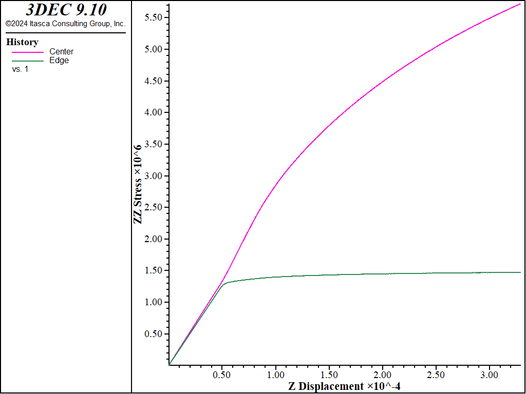
The axial (\(z\)-direction) stress-displacement response is monitored at the center and outer boundary in the grid. The results are shown in the figure below.

Figure 1: Stress-displacement plots for compression of Mohr-Coulomb material. Response is shown for an interior location (upper curve) and a boundary location (lower curve).

The test is now repeated with the strain-softening model.

Compression test on strain-softening material

model new
model large-strain off

; Create block and zones
block create drum center-1(0,0,0) center-2 (0,0,2) ...
                     radius-1 1 radius-2 1 edges 16
block zone generate-new maximum-edge 0.25

; Constitutive Model and properties
block zone cmodel assign strain-softening
block zone property density 2500 bulk 1.19e10 shear 1.1e10
block zone property cohesion 2.72e5 friction 44 tension 2e5
block zone property table-cohesion 'coh' table-friction 'fri'
table 'coh' add (0,2.72e5) (1e-4,2e5) (2e-4,1.5e5) (3e-4,1.03e5) (1,1.03e5)
table 'fri' add (0,44) (1e-4,42) (2e-4,40) (3e-4,38) (1,38)

; Boundary Conditions
block gridpoint apply velocity (0, 0, 1e-3) range position-z 0 
block gridpoint apply velocity (0, 0, -1e-3) range position-z 2

; Histories
block history displacement-z position (0,0,0)
block history stress-zz position (0,0,1)
block history stress-zz position (1,0,1)

model step 20000
model save 'Softening'

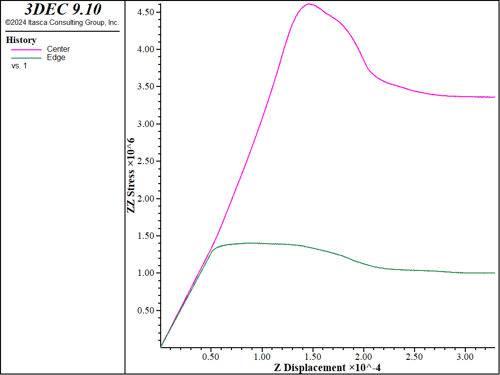
The horizontal stress-displacement response is monitored again, as shown in the image below. This test produces distinct peak and residual failure stress levels.

Figure 2: Stress-displacement for compression test of strain-softening material (similar monitoring points to those in the previous image).

The strain-softening model assumes both a brittle softening (due to reduction in cohesion) and a gradual softening (due to a reduction in friction angle). The selection of the properties is discussed further in Material Properties.

Comparison of the two images above illustrates the different responses of the two models. The initial response up to the onset of failure is identical, but post-failure behavior is quite different. Clearly, more data are required to use the strain-softening model and, typically, the softening model must be calibrated for each specific problem.

The effect of confinement on the “measured” response is also demonstrated from these plots. The history recorded in the middle of the grid shows that a higher stress level develops in the center of the model than at the free side. The location of monitoring points should correspond as closely as possible to the location of measurements in the physical problem.

The Effect of Water

Geologic materials generally appear weaker when the pore spaces contain a pore fluid under pressure. This is represented in 3DEC by the incorporation of an effective stress that accounts for the presence of pore pressure in a zone. The pore pressures in 3DEC are taken to be positive in compression. Thus, the effective stress \(\sigma^{\prime}\) is related to the total stress \(σ\) and pore pressure \(p\) by

\[\sigma^{\prime} = \sigma + p\]

Effective stresses are used in all of the plasticity models.

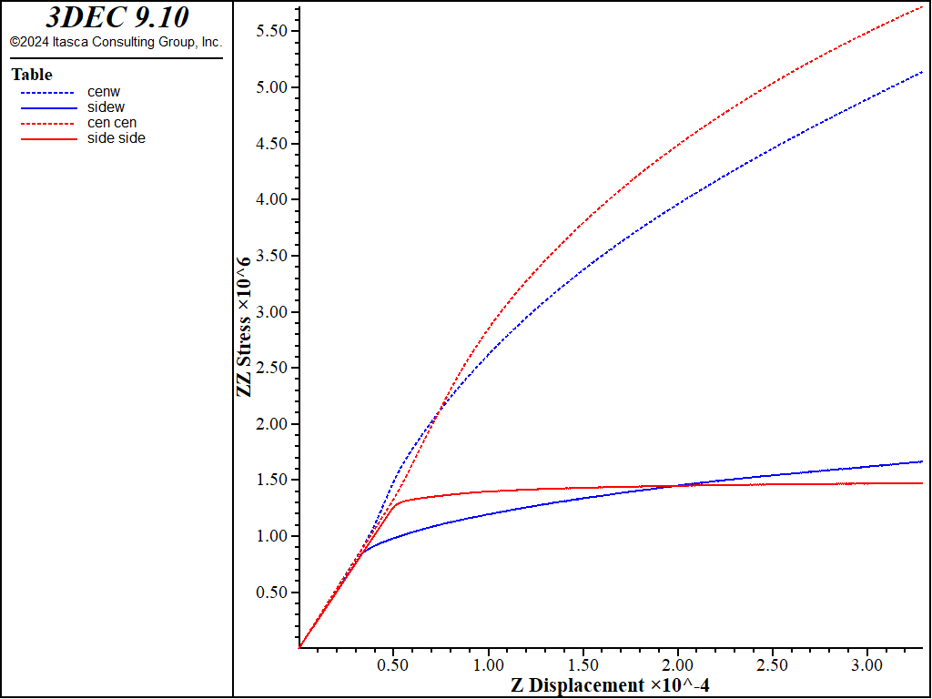
The effect of water can be seen by repeating the strain-softening example in the preceding topic, but with constant pore pressure in the zones (i.e., an undrained compression test). Add the command

; Initial Conditions
block gridpoint initialize pore-pressure 1e5

to the example before stepping. The lower strength is seen below.

Figure 3: Stress-displacement plots for compression test of Mohr-Coulomb material at constant pore pressure.

Ways to Implement Constitutive Models

There are several different ways a constitutive model can be implemented in 3DEC. The standard way is to invoke one of the built-in models with the block zone cmodel assign command. The user-defined models described in Writing New Constitutive Models are also invoked with the block zone cmodel assign command.

The source codes for the built-in models are included in the “\pluginfiles\cmodels” sub-directory, and are also copied to the application data location provided by the user the first time the program is launched. These files should be reviewed as examples for users who wish to write and implement their own models. User-defined models are written in C++ and are implemented as DLLs that are loaded with the 3DEC executable file in the same manner as the built-in models.[2] (See Writing New Constitutive Models.)

Often, it is desirable to modify an existing constitutive model (either a built-in model or a user-defined model) to make material properties dependent on other model parameters. There are three ways this can be done:

1. change properties of the built-in model via a FISH function that scans all the zones and is called at a specified step increment (say, every ten steps);[3]

2. change properties in a user-defined constitutive model function at every step by reference to a formula; or

3. change properties via look-up tables (with table commands) that modify strength properties as a function of plastic strain for the built-in strain-softening and double-yield models.

The third approach is the most efficient way to change properties in a 3DEC model. The first approach is the least efficient.

Endnotes

[1]

Users can create their own constitutive models as DLLs by following the procedures given in Writing New Constitutive Models. Also available are nine optional models that simulate viscoelastic and viscoplastic, time-dependent (creep) behavior (see Creep Model Group).

[2]

Note that this approach differs from the FISH constitutive model used in two-dimensional FLAC. With the DLL approach, user-defined models run at the same calculational speed as built-in models.

[3]

Note that increasing stiffness properties requires that a general update be performed in order to preserve stability.