FLAC3D Theory and Background • Fluid-Mechanical Interaction

Semi-confined Aquifer (FLAC2D)

Note

The project file for this example is available to be viewed/run in FLAC2D. The project’s main data files are shown at the end of this example.

Fluid leakage into a shallow semi-confined aquifer can be modeled with FLAC2D using the zone face apply leakage command. This is demonstrated for the example defined by the sketch in Figure 1. The aquifer has a length \(L\), height \(H\), and rests on an impermeable base. Fluid flow obeys Darcy’s law; the mobility coefficient \(k\) is homogeneous and isotropic. The semi-permeable top layer has permeability \(k_*\), and thickness \(H_*\). The effect of gravity is neglected in this example. Fluid pressure at the top of the leaky layer is constant and equal to \(p_*\). The lateral fluid-flow conditions correspond to a constant pressure \(p_0\) at the left boundary, and \(p_1\) at the right.

The objective is to determine the steady-state pore-pressure profile and total leakage into the aquifer. The general solution of pore pressure for a shallow semi-confined aquifer has the form (see Strack 1989)

(1)\[p - p_* = Ae^{x/\lambda} + Be^{-x/\lambda}\]

where \(\lambda\) is the seepage factor, which has the dimension of length and is defined as \(\lambda = \sqrt{k H H_*/k_*}\); \(A\) and \(B\) are constants determined from the pressure boundary conditions.

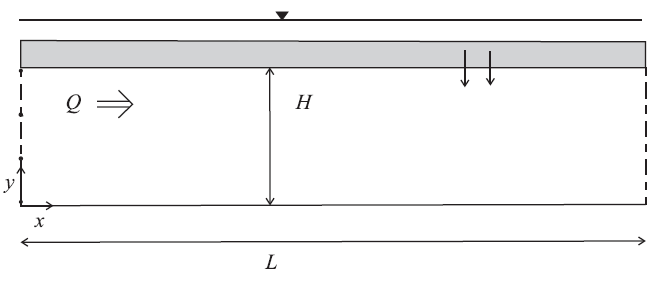
Figure 1: Shallow semi-confined aquifer.

The boundary conditions for this problem are

\(p = p_0\)	at	\(x = 0\)
\(p = p_1\)	at	\(x = L\)

The pore pressure solution is

(2)\[p = A e^{x/\lambda} + Be^{-x/\lambda} + p_*\]

where

(3)\[A = {{(p_1 - p_*)e^{L/\lambda} - (p_0 - p_*)} \over {e^{2L/\lambda} - 1}}\]

(4)\[B = {{(p_0 - p_*)e^{2L/\lambda} - (p_1 - p_*)e^{L/\lambda}} \over {e^{2L/\lambda} - 1}}\]

The steady state discharge over the height of the aquifer is obtained from Darcy’s law:

(5)\[Q_x = k H {dp \over dx}\]

After differentiation of Equation (2) with respect to \(x\), and substitution into Equation (5), we obtain

(6)\[Q = {{kH} \over \lambda}\Bigl\lbrack A e^{x/\lambda} - B e^{-x/\lambda} \Bigr\rbrack\]

The total amount of leakage into the aquifer is, by continuity of flow, equal to the difference between the discharge leaving at \(x\) = \(L\) and that entering at \(x\) = 0. Using Equation (6), we obtain, after some manipulation,

(7)\[Q_x = 2{{kH} \over \lambda} {{e^{L/\lambda} - 1} \over {e^{L/\lambda} + 1}}\Bigl\lbrack {p_0+p_1 \over 2} - p_* \Bigr\rbrack\]

Equation (6) and Equation (7) are used for comparison to the FLAC2D solution.

The FLAC2D data file for this problem is listed in “SemiConfinedAquifer.dat”. The analytical solution is programmed in FISH as part of the data file. The FLAC2D model is a 21 zone by 1 zone mesh with a constant pore pressure of \(p_0\) = 20 kPa applied at the left boundary, \(x\) = 0, and a constant pore pressure of \(p_1\) = 10 kPa applied at the right boundary, \(x\) = 20 m. A leaky aquifer boundary condition is applied along the top boundary of the model, \(y\) = 1 m, using the zone face apply leakage command. The pore pressure at the top is \(p_*\) = 1.8 kPa, and the leakage coefficient \(h\) (see this equation), is evaluated to be \(k_*/H_*\) = 2.98 × 10^-9 m³ /(N sec), based on the properties of the leaky layer. The properties for this problem are listed in the setup function. The fluid-flow calculation mode is turned on, the mechanical calculation mode is turned off, and the simulation is run until steady-state flow is reached.

The FISH function checkit compares the amount of leakage calculated by FLAC3D to the solution of (7) at steady-state flow. The difference is printed (in a FISH dialog message) to be 0.03%. The analytical and numerical pore pressure profiles recorded along the base of the model, from \(x\) = 0 to \(x\) = 20, are compared in Figure 2.

The same model is run twice more - once with the implicit servo active and once using the zone fluid steady-state command to immediately find the steady state. The pore-pressure distribution of all three methods are the same to within 0.1%.

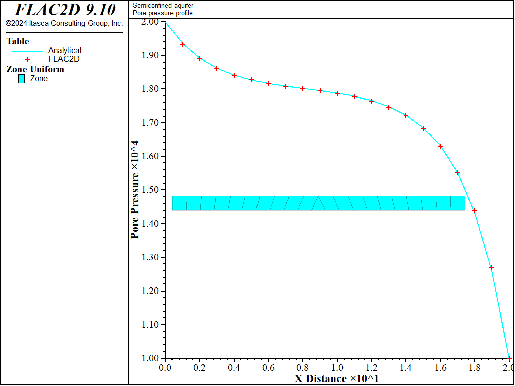
Figure 2: Pore pressure profile.

Reference

Strack, O. D. L. Groundwater Mechanics. New Jersey: Prentice Hall (1989).

pagebreak

Data File

SemiConfinedAquifer.dat

; file for 'Semiconfined aquifer'
model new
model title 'Semiconfined aquifer'
; Geometry
;zone create quadrilateral point 0 (0,0) point 1 (20,0) point 2 (0,1) point 3 (20,1) size 20 2
program call 'GeomTriangle' ; a geometry with triangle
zone nodal-mixed-discretization off ; nmd should be off as it is not implemented yet for 2D fluid
zone face skin
; Constitutive model and properties
model configure fluid-flow
zone fluid property porosity=0.04 mobility-coefficient=2e-8
zone fluid property fluid-modulus 2e9
; --- boundary conditions ---
zone face apply leakage 1.8e4 3e-9 range group 'Top'
zone gridpoint fix pore-pressure 2e4 range group 'West'
zone gridpoint fix pore-pressure 1e4 range group 'East'
model save 'start'

; --- Explicit fluid flow solution ---
model solve-fluid time 1
model save 'confaquifer'

; --- Implicit fluid flow solution ---
model restore 'start'
zone fluid implicit servo on 
model solve-fluid time 1
model save 'confaquifer-imp'

; --- Steady state flow solution ---
model restore 'start'
zone fluid steady-state
model save 'confaquifer-steady'