FLAC3D Theory and Background • Fluid-Mechanical Interaction

Unsteady Groundwater Flow in a Confined Layer (FLAC2D)

Note

To view this project in FLAC2D, use the menu command Help ► Examples…. The project’s main data files are shown at the end of this example.

A long embankment of width \(L\) = 100 m rests on a shallow saturated layer of soil. The width (\(L\)) of the embankment is large in comparison to the layer thickness, and its permeability is negligible when compared to the permeability, \(k\) = 10^-12 m²/(Pa sec), of the soil. The Biot modulus for the soil is measured to be \(M\) = 10 GPa. Initial steady-state conditions are reached in the homogeneous layer. The purpose is to study the pore-pressure change in the layer as the water level is raised instantaneously upstream by an amount \(H_0\) = 2 m. This corresponds to a pore-pressure rise of \(p_1 = H_0 {\rho}_w g\) (with the water density \({\rho}_w\) = 1000 kg/m³ and acceleration of gravity \(g\) = 10 m/s²) at the upstream side of the embankment. Figure 1 shows the geometry of the problem:

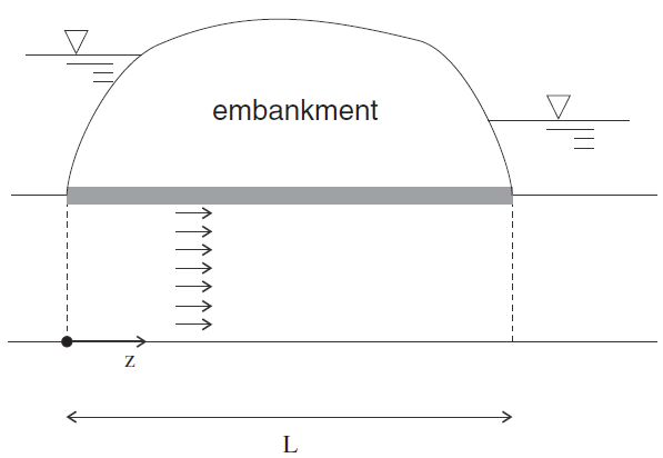
Figure 1: Confined flow in a soil layer.

The flow in the layer may be assumed to be one-dimensional. The model has width \(L\). The excess pore pressure, \(p\), initially zero, is raised suddenly to the value \(p_1\) at one end of the model. The corresponding analytical solution has the form

\[\hat{p}(\hat{z},t)\ =\ 1 - \hat{z} - {2 \over {\pi}} \sum_{n=1}^\infty e^{- n^2\pi^2 \hat{t}}\left({\sin {n \pi \hat{z}} \over n}\right)\]

where the \(z\)-axis is running along the embankment width and has its origin at the upstream side, \(\hat{p} = {p\over p_1}\), \(\hat{z} = {z \over {L}}\), \(\hat{t} = c t/L^2\), and \(c = M k\).

In the FLAC2D model, the layer is defined as a column of 25 zones. The excess pore pressure is fixed at the value of 2 × 10⁴ Pa at the face located at \(z\) = 0, and at zero at the face located at \(z\) = 100 m. The model grid is shown in Figure 2.

The analytical solution is programmed as a FISH function for direct comparison to the numerical results at selected fluid-flow times corresponding to \(\hat{t}\) = 0.05, 0.1, 0.2 and 1.0. The analytical and numerical pore-pressure results for these times are stored in tables.

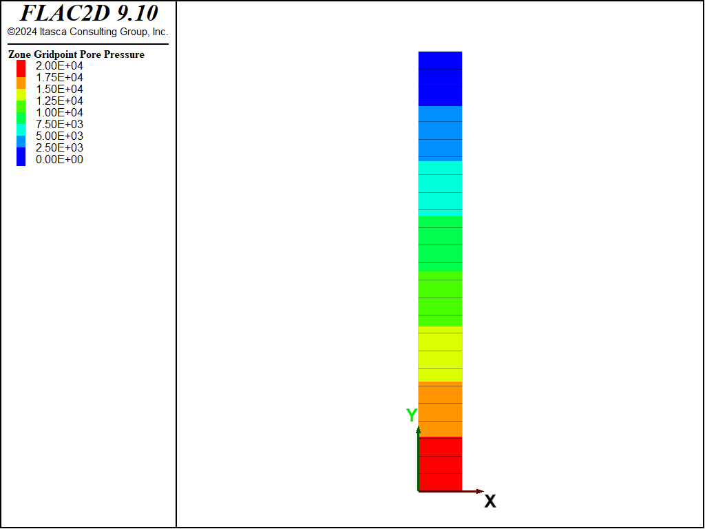
Figure 2: FLAC2D grid for fluid flow in a confined soil layer.

UnsteadyGroundwaterFlowConfinedLayer.dat contains the FLAC2D data file for this problem, using the implicit servo to automatically switch from explicit to implicit and increase the implicit timestep. SteadyGroundwaterFlowConfinedLayer.dat contains the data file using the zone fluid steady-state command to immediately find the steady state solution.

The comparison of analytical and numerical excess pore pressures at four fluid-flow times for the transient solution is shown in Figure 3. Normalized excess pore pressure (\(p/p_1\)) is plotted versus normalized distance (\(z/L\)) in the figure, where Tables 2, 4, and 6 contain the analytical solution for excess pore pressures, and Tables 1, 3, and 5 contain the FLAC2D solutions. The four flow times are 5 × 10⁴, 10⁵, 2 × 10⁵, and 10⁶ seconds. Steady-state conditions are reached by the last time considered. The difference between analytical and numerical pore pressures at steady state is less than 0.2%.

break

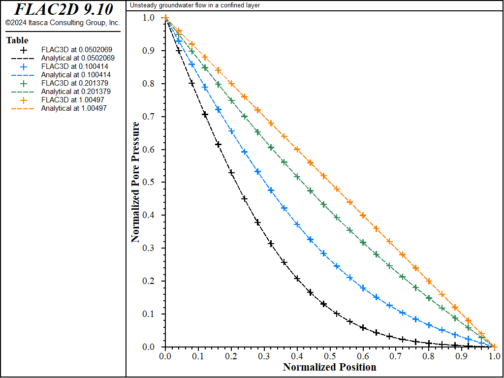
Figure 3: Comparison of excess pore pressures (analytical values = lines; numerical values = crosses).

Data File

UnsteadyGroundwaterFlowConfinedLayer.dat

model new
model title 'Unsteady groundwater flow in a confined layer'
zone create quadrilateral size 1 25 point 1 (10 0) point 2 (0 100) point 3 (10 100)
zone face skin
; --- fluid flow model ---
model configure fluid-flow
zone fluid property mobility-coefficient 1e-12
zone fluid property biot-modulus 1e10
zone face apply pore-pressure 2e4 range group 'Bottom'
zone face apply pore-pressure 0   range group 'Top'
; --- settings ---
zone fluid implicit servo on 
zone results pore-pressure on
; --- solve ---
model solve-fluid time 5e4
model results export 'confinedlayer-005'
model solve-fluid time 5e4 ; total 10e4
model results export 'confinedlayer-010'
model solve-fluid time 10e4 ; total 20e4
model results export 'confinedlayer-020'
model solve-fluid time 80e4 ; total 100e4
model results export 'confinedlayer-100'
model save 'confinedlayer'

SteadyGroundwaterFlowConfinedLayer.dat

model new
zone create quadrilateral size 1 25 point 1 (10 0) point 2 (0 100) point 3 (10 100)
zone face skin
; --- fluid flow model ---
model configure fluid-flow
zone fluid property mobility-coefficient 1e-12
zone face apply pore-pressure 2e4 range group 'Bottom'
zone face apply pore-pressure 0   range group 'Top'

zone fluid steady-state

model save 'confinedlayer-steady'