Laterally Loaded Pile
Problem Statement
Note
To view this project in FLAC2D, use the menu command . The main data files used are shown at the end of this example. The remaining data files can be found in the project.
A vertical pile is subjected to a lateral displacement at its top. The pile is pushed in one direction, then the loading is reversed and the pile is pushed in the opposite direction. This loading cycle is performed for the case of no normal gap present, and then for 100% of the gap effective. The results demonstrate the response of the pile structural elements to lateral loading both with and without the effect of a gap between the pile and the medium. The top node of the pile is marked with the group name Top.
In the FLAC3D data file, the pile (composed of 8 pile elements) is created in the center of
the soil block such that the top pile node is one meter above the soil surface (see Figure 1). We wish to apply to the top node a constant lateral velocity of 1 × 10⁻⁸.
We specify this nodal velocity condition with the structure node initialize velocity
(0,-1e-8) local range group 'Top' command.
We must also specify the appropriate velocity-fixity condition at this node with the
structure node fix command, which requires specification of fixity directions in the
node-local system, not the global system. Because the top node is used by a pile element, its
node-local system will be oriented such that the \(x\)-axis is aligned with the pile axis,
and the \(y\)-axis is aligned perpendicular to the pile. In our model, the node-local
system of the top node is oriented such that the \(x\)-axis points in the negative global
\(y\)-direction, the \(y\)-axis points in the positive global \(x\)-direction. The orientation of the
node-local system can be visualized with the “Pile” plot item by setting the “System” attribute
to “Node”.
Note that this orientation is set automatically at the start of a set of cycles, or when the
model cycle 0 command is executed. Therefore, we fix the lateral velocity to
remain constant with the commands
struct node fix velocity-y range group 'Top' ; fix velocities in lateral plane
We wish to monitor the applied load acting at the top node and plot this value versus the displacement of the top node. If the loading is applied in a quasi-static fashion, then the applied load acting at the top node will equal the shear force acting at the top end of the top pile element. The shear forces are expressed using the (see force-moment sign convention).
The applied lateral load can then be monitored with the structure pile history command:
struct pile history name='force' force-y component-id 1 ; shear force at top
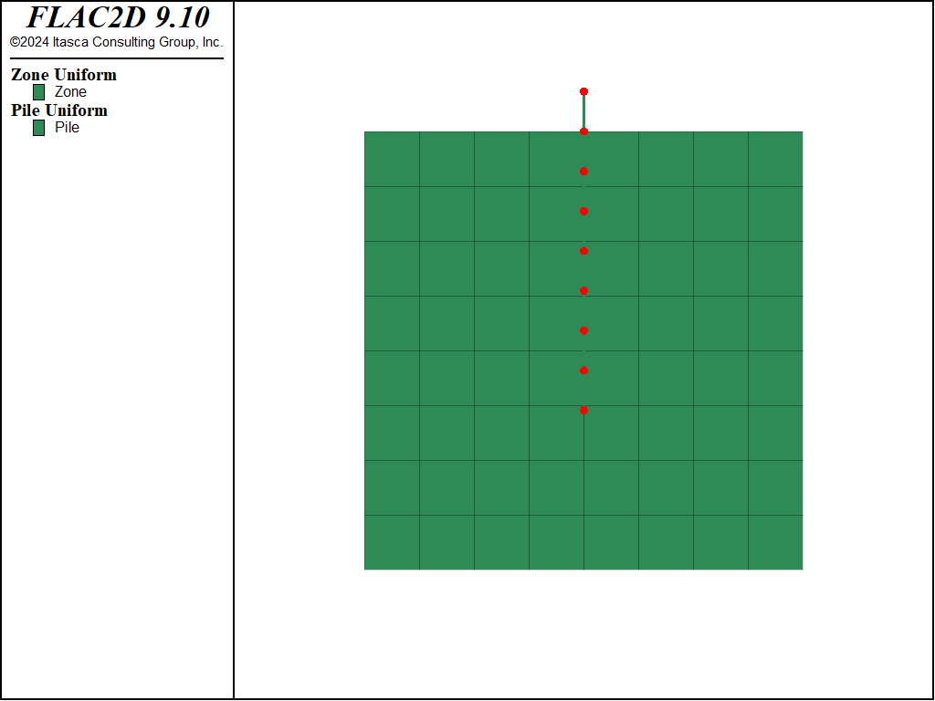
Figure 1: Soil block and vertical pile.
The \(y\)-component of the applied displacement can be monitored with
separate structure node history commands;
For this problem, the cohesion and friction of the normal coupling spring are set to 0.01 MN/m
and zero, respectively. The no-gap case is run by specifying coupling-gap-normal
off in the structure pile property command. The full-gap case is run by
specifying coupling-gap-normal on. Figure 2
shows the normal load at the pile top versus displacement for the no-gap case, and
Figure 3 shows the results for the full-gap case. During the lateral
loading, the limiting normal force is the same for both cases. However, the normal load versus
displacement histories are different. In the model with a full gap, it is necessary to close the
gap before the force with opposite direction is generated. The pile is unloaded when it returns
to its initial position.
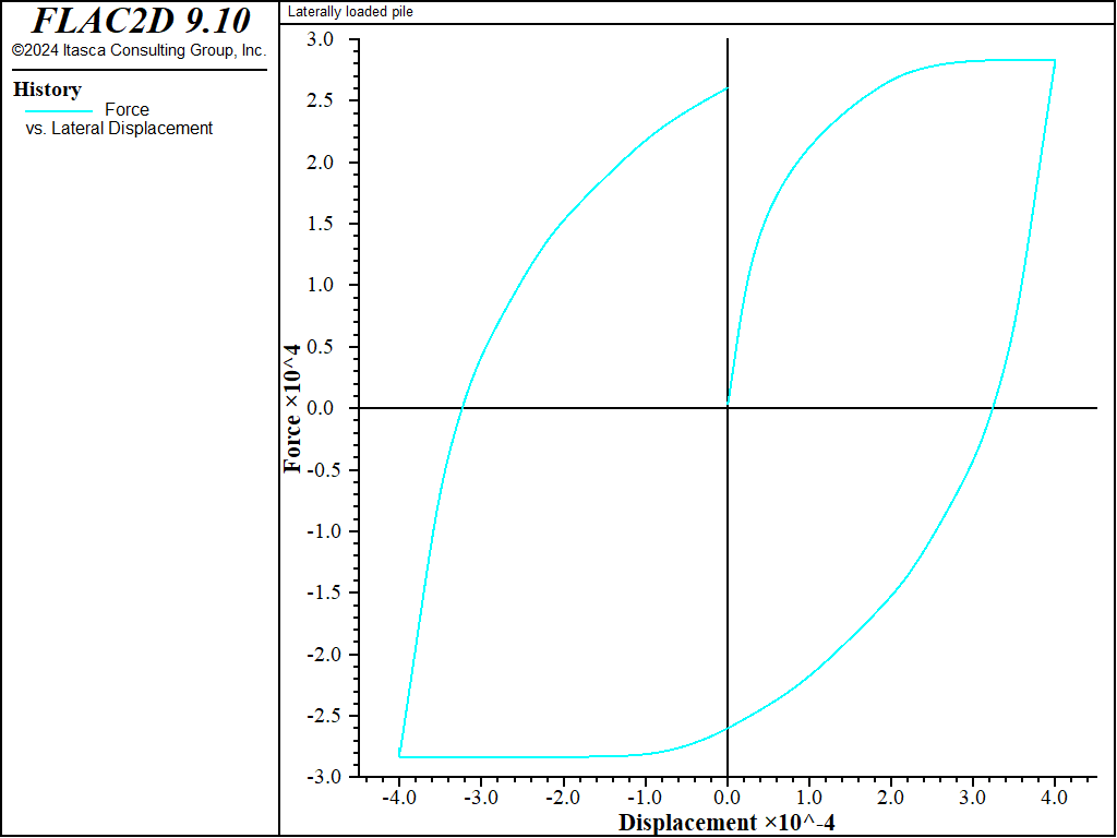
Figure 2: Shear load at top of pile versus lateral displacement for no gap.
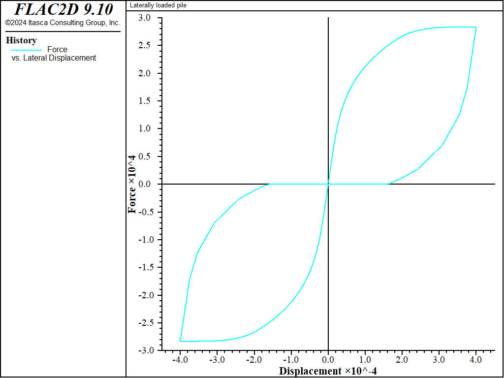
Figure 3: Shear load at top of pile versus lateral displacement for full gap.
Additional information about the system behavior can be learned by studying the model at the end of the first stage of loading, when the initial applied displacement is 0.4 mm. At this stage, the upper portion of the pile is compressing the soil in the \(x\)-direction, while the lower portion of the pile is compressing the soil in the negative \(x\)-direction. The plots of nodal displacement, bending moment in the pile, and stress and yield state of the normal coupling springs (see Figure 4 and Figure 5) confirm this loading mode and indicate that the normal coupling springs above and below the load-reversal point are yielding. The normal stress is zero over the top element, because the top node is above the soil surface. From Figure 4 it can be seen that the normal stress at the yielding nodes equals 3.185 kPa. This equals normal cohesion, \(c_s\), divided by perimeter, \(p\), as it should. The pile responses can also be accessed via FISH.
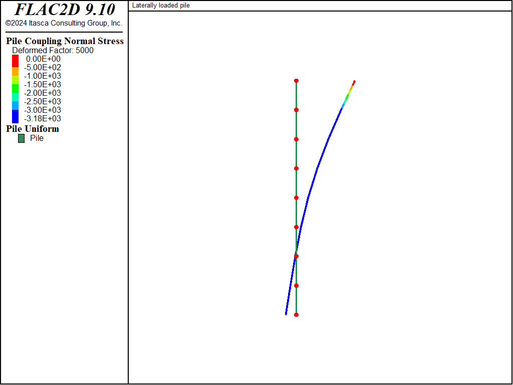
Figure 4: Stress and yield state of normal coupling springs (undeformed and deformed with deformation factor of 5000, end of first loading stage, gap on).
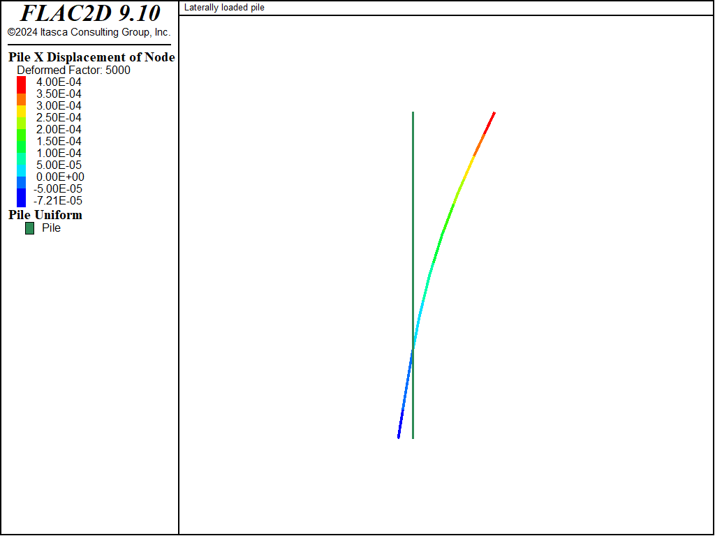
Figure 5: Moment distribution (undeformed and deformed with deformation factor of 5000, end of first loading stage, gap on).
Data File
LaterallyLoaded.dat
model new
model large-strain off
model title "Laterally loaded pile"
; Create zones
zone create quadrilateral size 8 8 edge=11
zone face skin ; Label model boundaries
; Assign material model and properties
zone cmodel assign elastic
zone property bulk=5e9 shear=1e9 density=2000
; Boundary conditions
zone face apply velocity-normal 0 range group 'East' or 'West'
zone face apply velocity-normal 0 range group 'Bottom'
; Initial conditions
model gravity 10
zone initialize-stresses ratio 0.6
model solve ratio-local 1e-4 ; Should be instant
; =======================================================
; Create a pile in the center of the soil block
structure pile create by-line (5.5,12.0) (5.5,4.0) segments=8
structure node group 'Top' range position-y 12 ; Tag top node
structure pile property young=8.0e10 poisson=0.30 cross-sectional-area=0.7854 ...
            moi=4.91e-2 ...
            perimeter=3.14 ...
            coupling-stiffness-shear=1.3e11 coupling-cohesion-shear=1.0e10 ...
            coupling-friction-shear=0.0 coupling-stiffness-normal=1.3e09   ...
            coupling-cohesion-normal=1.0e04 coupling-friction-normal=0.0   ...
            coupling-gap-normal=off
; =======================================================
structure pile history name='force' force-y component-id 1 ; shear force at top
structure node history name='disp' displacement-y local component-id 1; lateral displacement
; =======================================================
structure mechanical damping combined-local
structure node fix velocity-y range group 'Top' ; fix velocities in lateral plane
; move (+)
structure node initialize velocity (0,1.0e-8) local range group 'Top'
model save 'Initial'
; =======================================================
; Run no-gap case
; =======================================================
model cycle 40000  ; disp of +4e-4
model save 'NoGap-1'
; move (-)
structure node initialize velocity (0,-1.0e-8) local range group 'Top'
model cycle 80000  ; disp of -8e-4
model save 'NoGap-2'
; move (+)
structure node initialize velocity (0,1.0e-8) local range group 'Top'
model cycle 40000                                           ; disp of +4e-4
model save 'NoGap-Final'
; =======================================================
; Run full-gap case
; =======================================================
model restore 'Initial'
structure pile property coupling-gap-normal on
model cycle 40000  ; disp of +4e-4
model save 'FullGap-1'
; move (-) diag-dir
structure node initialize velocity (0,-1.0e-8) local range group 'Top'
model cycle 80000  ; disp of -8e-4
model save 'FullGap-2'
; move (+) diag-dir
structure node initialize velocity (0,1.0e-8) local range group 'Top'
model cycle 40000                                           ; disp of +4e-4
model save 'FullGap-Final'
| Was this helpful? ... | Itasca Software © 2024, Itasca | Updated: Aug 13, 2024 |
