Pumping Test in a Single Horizontal Fracture
Note
To view this project in 3DEC, use the menu command . The main data files used are shown at the end of this example. All data files are found in the project.
Problem Statement
The pressure drawdown in a single horizontal fracture due to constant flow pumping is analysed here. No hydro-mechanical coupling is considered. Fluid pressures at different times and locations are compared to analytical solutions.
Analytical Solution
The fracture is used to represent a confined aquifer of thickness b, where analytical solutions are well established in hydrogeology (Figure 1).
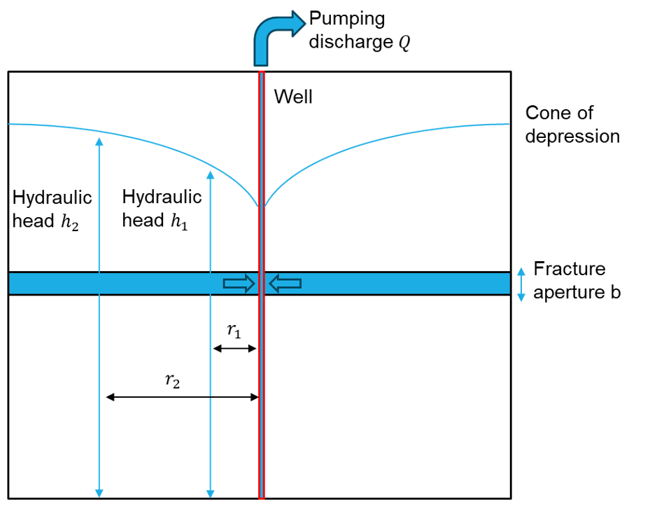
Figure 1: Geometry of the problem of pressure drawdown in a single horizontal fracture due to constant flow pumping.
While flow is unsteady, the solution of Theis [1] describes the hydraulic head (i.e pressure) drawdown \(h(r,t)\) at a distance r from pumping and time t:
where
and
where T is the transmissivity (units of \(Length^2/Time\)) and S is the storage (units of \(1/Length\)).
Once flow is steady, the solution of Thiem [2] describes the hydraulic head difference \((h_2 - h_1)\) between two points distant from \(r_1\) and \(r_1\) of the puming well:
3DEC Model
The geometry of the 3DEC model used for this analysis is shown in Figure 2. The model consists of two blocks separated by a horizontal joint plane of size 50m. The target mesh size is 2 m. A vertical well is created as a geometry object (for visualization only).
Water properties are used as shown below:
Property |
Value |
|---|---|
Fluid density (\(\rho_f\)) |
1000 kg/m^3 |
Fluid bulk modulus (\(K_f\)) |
2.2 GPa |
Fluid viscosity (\(\mu_f\)) |
0.001 Pa.s |
The transmissivity can be calculated by:
where b is the joint aperture. For \(b = 2.3 \times 10^{-5}\) and the fluid properties above, this yields \(T = 1 \times 10^{-8} m^2/s\)
The storage can be calculated by:
for the values used in this example, \(S = 1.02743 \times 10^{-10}\)
Finally, a constant hydraulic discharge of \(Q = -10^{-7} m^3/s\) (negative value means pumping) is applied at the center of the fracture, while the hydraulic head is fixed to 100 m at the model boundaries.
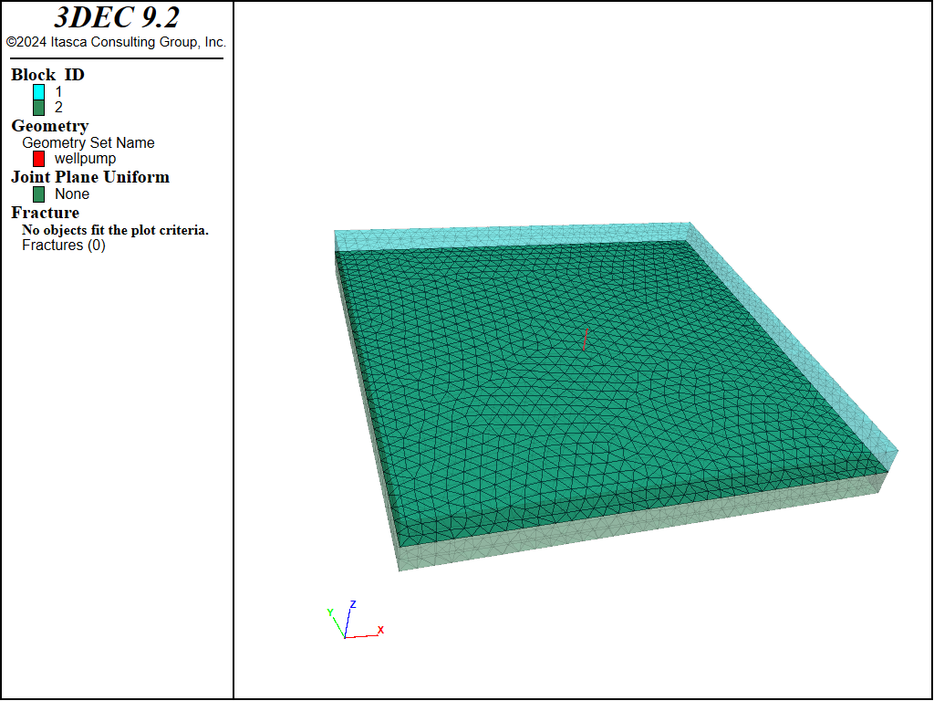
Figure 2: Geometry of the problem of pressure drawdown in a single horizontal fracture due to constant flow pumping.
Results and Discussion
Figure 3 shows the pore pressure field in the fracture plane.
Hydraulic drawdown is computed through time from solved pressure at flowknots and compared with Theis solutions. The comparison is shown in Figure 4.
Once a steady state is reached, the pressures are constant in all flowknots. The hydraulic head difference \((h_2 - h_1)\) between each pair of flowknots distant from \(r_1\) and \(r_2\) of the puming well are plotted in Figure 5, and show excellent agreemnt with Thiem solutions.
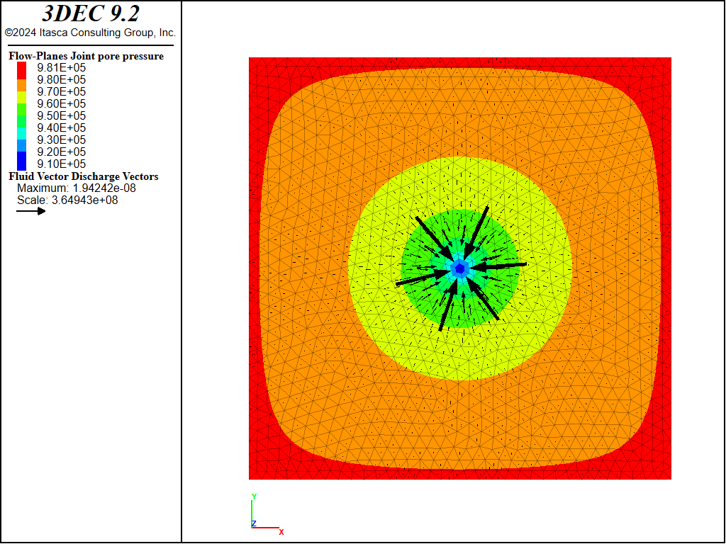
Figure 3: Pore pressure field in the fracture plane.
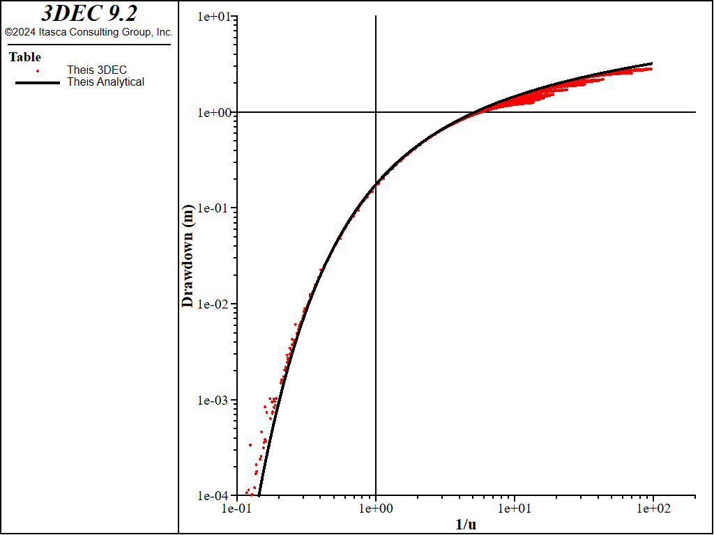
Figure 4: Comparison of 3DEC results with Theis analytical solution (transient flow).
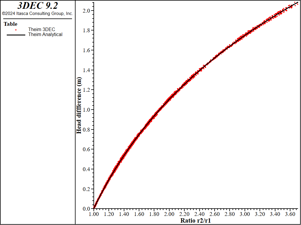
Figure 5: Comparison of 3DEC results with Thiem analytical solution (steady-state flow).
References
[1] Theis, C. V. (1935). The relation between the lowering of the piezometric surface and the rate and duration of discharge of a well using ground‐water storage. Eos, Transactions American Geophysical Union, 16(2), 519-524.
[2] Thiem, G. (1906). Hydrologische methoden.
Data Files
drawdown.dat
model new
model configure fluid-flow
model large-strain off

;------------------------------------------------
; Set simulation parameters
;------------------------------------------------
[domain_size=50]
[mesh_size=1.5]
[transmissivity=1e-8]
[hmax=100.]
[discharge=-1e-7]
[fbulk=2.2e9]
[fdens=1000.]
[fvisc=1e-3]
;------------------------------------------------

;------------------------------------------------
; Create units conversion functions
;------------------------------------------------
fish define convert_head_to_pp(head)
    return head*(fdens*9.81)
end
fish define convert_pp_to_head(pp)
    return pp/(fdens*9.81)
end
;------------------------------------------------

;------------------------------------------------
; Create variables
;------------------------------------------------
[aperture = ((12.*fvisc*transmissivity)/(fdens*9.81))^(1./3.)]
[ppmax = convert_head_to_pp(hmax)]
[storage = (fdens*9.81*aperture)/fbulk]
;------------------------------------------------

;------------------------------------------------
; Create model geometry
;------------------------------------------------
;create blocks and joint set
block create brick [-domain_size/2] [domain_size/2] ...
                   [-domain_size/2] [domain_size/2] ...
                   [-2*mesh_size] [2*mesh_size]

; cut joint for fluid flow
block cut joint-set dip 0 dip-direction 90

;create well for visualization
geometry set 'wellpump'
geometry edge create by-positions 0. 0. [2*mesh_size] 0. 0. [-2*mesh_size]

; mesh
block zone generate edgelength [mesh_size] fix 0 0 0

;------------------------------------------------

;------------------------------------------------
; Set properties
;------------------------------------------------
; set mechanical properties
block zone cmodel assign elastic
block zone property density 2500 shear 2e9 bulk 5e9
block contact jmodel assign mohr
block contact property stiffness-normal 1e10 stiffness-shear 1e10
; set fluid  properties
block fluid property bulk [fbulk]
block fluid property density [fdens]
block fluid property viscosity [fvisc]
; set flowplane properties
flowplane vertex property aperture-initial [aperture] ...
                          aperture-minimum [aperture] ...
                          aperture-maximum [aperture]
;------------------------------------------------

;------------------------------------------------
; Set boundary conditions
;------------------------------------------------
block insitu pore-pressure [ppmax]
flowknot apply pore-pressure [ppmax] range position-x [-domain_size/2]
flowknot apply pore-pressure [ppmax] range position-x [domain_size/2]
flowknot apply pore-pressure [ppmax] range position-y [-domain_size/2]
flowknot apply pore-pressure [ppmax] range position-y [domain_size/2]
flowknot apply discharge [discharge] ...
  range id [flowknot.id(flowknot.near(0,0,0))]
;------------------------------------------------

;------------------------------------------------
; Record histories
;------------------------------------------------
model history fluid time-total
fish define find_knots
  fk1 = flowknot.near(1,0,0)
  fk2 = flowknot.near(2,0,0)
  fk3 = flowknot.near(5,0,0)
  fk4 = flowknot.near(10,0,0)
  fk5 = flowknot.near(15,0,0)
end
[find_knots]

fish define drawdown1
    global drawdown1 = hmax - convert_pp_to_head(flowknot.pp(fk1))
    global drawdown2 = hmax - convert_pp_to_head(flowknot.pp(fk2))
    global drawdown5 = hmax - convert_pp_to_head(flowknot.pp(fk3))
    global drawdown10 = hmax - convert_pp_to_head(flowknot.pp(fk4))
    global drawdown15 = hmax - convert_pp_to_head(flowknot.pp(fk5))
end
fish history name 'drawdown1' drawdown1
fish history name 'drawdown2' drawdown2
fish history name 'drawdown5' drawdown5
fish history name 'drawdown10' drawdown10
fish history name 'drawdown15' drawdown15

;------------------------------------------------

; call functions to get analytical solution
program call 'theis.fis'
;------------------------------------------------

;------------------------------------------------
; Solve
;------------------------------------------------
model fluid active on
model fluid timestep fix 0.001
model mechanical active off
fish callback add compute_analytical_theis 1 interval 10
model cycle 10000
;------------------------------------------------

; compute steady-state solution
[compute_analytical_thiem]
theis.fis
;------------------------------------------------
; Theis solution (transient flow)
;------------------------------------------------
[global tab_ana_theis = table.create('Theis Analytical')]
[global tab_3dec_theis = table.create('Theis 3DEC')]
fish define factorial(n)
    local res=1.
    loop local i(1,n)
        res*=i
    endloop
    return res
end
fish define well_func(u,tol)
    local wu = -0.57721566 - math.ln(u)
    local i = 1
    local err =  tol + 1.0
    loop while err>tol
        local wu_new=0.
        if (i % 2) == 0
            wu_new = wu - u^i/(i*factorial(i))
        else
            wu_new = wu + u^i/(i*factorial(i))
        endif
        err = math.abs(wu_new - wu)
        wu = wu_new
        i = i + 1
    endloop
    return wu
end
fish define compute_analytical_theis
    time = fluid.time.total

    ; only calculate for every 10th point
    local count = 0
    loop foreach local fki flowknot.list
        count += 1
        if count % 10 # 0
          continue
        endif
        local r_fki = math.mag(flowknot.pos(fki))
        if r_fki==0 | r_fki>0.25*domain_size | time>5.
            continue
        endif
        local pp_fki = flowknot.pp(fki)
        local h_fki = convert_pp_to_head(pp_fki)
        local s_fki = hmax - h_fki
        local u_fki = (r_fki*r_fki*storage)/(4.*transmissivity*time)
        if u_fki=0. | u_fki>100.
            continue
        endif
        local theis = math.abs(discharge)/(4.*math.pi*transmissivity)
        theis *= well_func(u_fki,1e-12)
        table(tab_3dec_theis,1./u_fki)=s_fki
        table(tab_ana_theis,1./u_fki)=theis
    endloop
end

;------------------------------------------------
; Thiem solution (steady state flow)
;------------------------------------------------
[global tab_ana_theim = table.create('Theim Analytical')]
[global tab_3dec_theim = table.create('Theim 3DEC')]
fish define compute_analytical_thiem
    ; only calculate for every 10th point
    local count = 0
    loop foreach local fki flowknot.list
        count += 1
        if count % 10 # 0
          continue
        endif
        local r_fki = math.mag(flowknot.pos(fki))
        if r_fki==0 | r_fki>0.25*domain_size
            continue
        endif
        local pp_fki = flowknot.pp(fki)
        local h_fki = convert_pp_to_head(pp_fki)
        loop foreach local fkj flowknot.list
            local r_fkj = math.mag(flowknot.pos(fkj))
            if r_fkj==0 | r_fkj>0.333*domain_size
                continue
            endif
            local pp_fkj = flowknot.pp(fkj)
            local h_fkj = convert_pp_to_head(pp_fkj)
            local head_diff = math.abs(h_fkj-h_fki)
            local rad_ratio = r_fkj/r_fki
            if rad_ratio<1.
                continue
            endif
            local thiem = math.abs(discharge)*math.ln(rad_ratio)
            thiem /= (2.*math.pi*transmissivity)
            table(tab_3dec_theim,rad_ratio)=head_diff
            table(tab_ana_theim,rad_ratio)=thiem
        endloop
    endloop
end
Endnote
| Was this helpful? ... | Itasca Software © 2024, Itasca | Updated: Dec 05, 2024 |
