Partial Density Scaling for Dynamic Analysis
Density scaling is a technique used in 3DEC in quasi-static calculations that substantially improves the efficiency in obtaining solutions to large problems. In quasi-static problems, inertial forces are not important. The gridpoints’ masses can be scaled for optimal numerical convergence without affecting the solution. In dynamic analyses, however, global scaling cannot be used. Complex jointed systems often result in very small blocks and/or zones being created during the automatic meshing procedure. The small blocks/zones require very small timesteps for numerical stability of the explicit algorithm. This makes some dynamic solutions extremely time consuming. However, as these blocks/zones may be very small, with very small masses, it is possible to introduce some density scaling only for these blocks/zones in such a way that the change of the system inertia is negligible. This scheme of partial density scaling is implemented in 3DEC in such a way that the user controls the amount of scaling to be introduced. Given the timestep calculated by the code, the user specifies the desired timestep with the command block mechanical mass-scale dt. This command specifies that only the amount of density scaling required to achieve the timestep dt is to be applied to the system. When a model cycle command is given, a message indicating the number of gridpoint masses that were scaled, and the amount of additional mass introduced, is printed.
Example of Partial Density Scaling
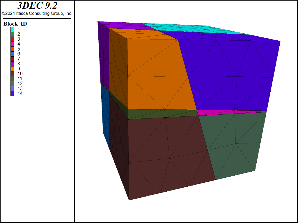
Figure 1 shows a simple block system with some low-thickness blocks. The timestep required for dynamic analysis without any scaling is 1.005e-6 seconds. Using partial density scaling, the timestep may be increased to 5e-6 seconds, while the total system mass is increased by only 5%.
This information is printed by 3DEC following the use of the block mechanical mass-scale command:
no. scaled g.p. masses = 68
min. g.p. scaling factor = 4.038E-02
max. g.p. scaling factor = 1.000E+00
min. g.p. added mass = 0.000E+00
max. g.p. added mass = 3.103E-05
min. block added mass = 0.000E+00
max. block added mass = 1.938E-04
total added mass in model = 8.202E-04
total real mass in model = 1.920E-02
added mass / real mass = 4.272E-02

Figure 1: View of model with small, thin blocks.
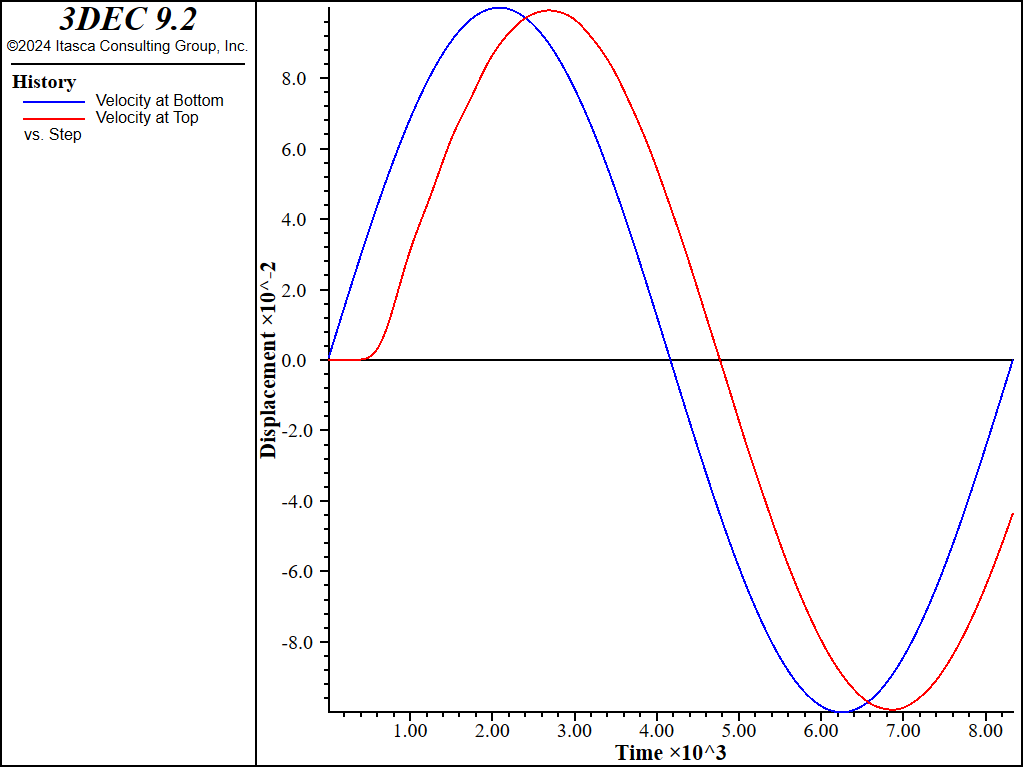
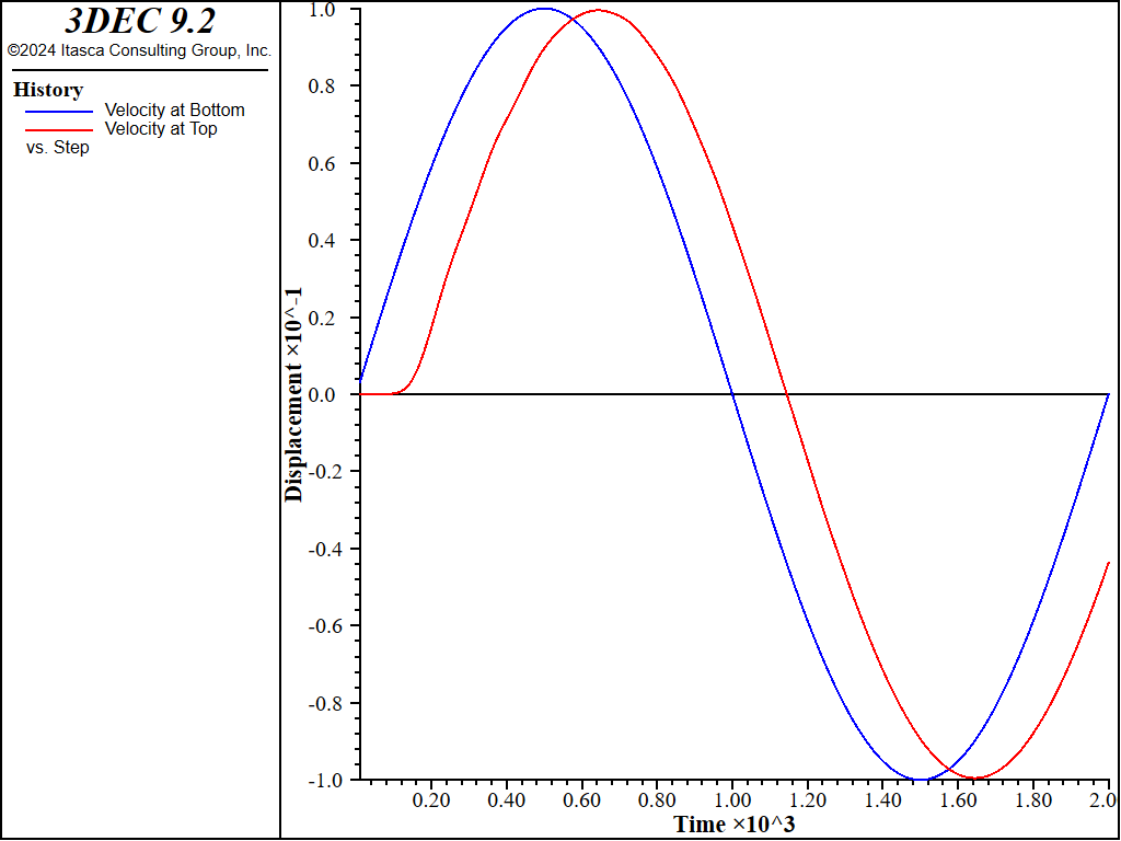
The effect of this amount of partial density scaling was checked by comparing the system response to a sinusoidal shear applied at the base of the model. A viscous boundary condition was applied to the top of the model to simulate an extended medium. Figure 2 shows the \(x\)-velocity applied at the base, and the velocity obtained at the top of the model, obtained in the run without scaling. Figure 3 shows the same quantities for the run with partial density scaling, with a timestep about 5 times larger. It can be seen that the wave propagation is not affected by the small amount of scaling introduced.

Figure 2: Velocities at the bottom and top of the model, for analysis without any density scaling.

Figure 3: Velocities at the bottom and top of the model, for analysis with partial density scaling.
Data File - No Scaling
;-----------------------------------------------------------------------
; Dynamic Analysis - no density scaling
;-----------------------------------------------------------------------

model new
model title "Dynamic Analysis - no density scaling"

model configure dynamic
model large-strain on

;geometry
block create brick -1,1 -1,1 -1,1
block cut joint-set dip 5 dip-direction 45 origin 0 0 0
block cut joint-set dip 10 dip-direction 40 origin 0 0 0
block cut joint-set dip 70 dip-direction 95
block cut joint-set dip 80 dip-direction 10

; zones
block zone generate edgelength 0.5
block zone cmodel assign elastic
block zone property density 0.0024 bulk 33333 shear 20000

; joints
block contact jmodel assign elastic
block contact property stiffness-normal 500000 stiffness-shear 500000
block contact material-table default property stiffness-normal 500000 ...
                                          stiffness-shear 500000


; off by default forigin mechanical analysis
;block mechanical mass-scale off

[freq = 100.0]
fish define sin_
  sin_ = math.sin(2.0*math.pi*mech.time*freq)
end

; boundary conditions
block gridpoint apply viscous range position-z 1
block gridpoint apply velocity-x 0.1 fish sin_ range position-z -1
block gridpoint apply velocity-y 0 velocity-z 0 range position-z -1
block gridpoint apply velocity-y 0 velocity-z 0 range position-x -1
block gridpoint apply velocity-y 0 velocity-z 0 range position-x 1
block gridpoint apply velocity-y 0 velocity-z 0 range position-y -1
block gridpoint apply velocity-y 0 velocity-z 0 range position-y 1

; histories
model history mechanical unbalanced-maximum
block history name 'Velocity at Bottom' velocity-x position -1 -1 -1
block history name 'Velocity at Top' velocity-x position -1 -1 1
model history name 'Time' dynamic time-total

model solve time-total 0.01
model save "zp2no"
Data File - Partial Scaling
;-----------------------------------------------------------------------
; Dynamic Analysis - no density scaling
;-----------------------------------------------------------------------

model new
model random 10000
model title "Dynamic Analysis - no density scaling"

model configure dynamic
model large-strain on

;geometry
block create brick -1,1 -1,1 -1,1
block cut joint-set dip 5 dip-direction 45 origin 0 0 0
block cut joint-set dip 10 dip-direction 40 origin 0 0 0
block cut joint-set dip 70 dip-direction 95
block cut joint-set dip 80 dip-direction 10

; zones
block zone generate edgelength 0.5
block zone cmodel assign elastic
block zone property density 0.0024 bulk 33333 shear 20000

; joints
block contact jmodel assign elastic
block contact property stiffness-normal 500000 stiffness-shear 500000
block contact material-table default property stiffness-normal 500000 ...
                                          stiffness-shear 500000

; partial scaling, maximum timestep 5e-6
block mechanical mass-scale timestep 5e-6

[freq = 100.0]
fish define sin_
  sin_ = math.sin(2.0*math.pi*mech.time*freq)
end

; boundary conditions
block gridpoint apply viscous range position-z 1
block gridpoint apply velocity-x 0.1 fish sin_ range position-z -1
block gridpoint apply velocity-y 0 velocity-z 0 range position-z -1
block gridpoint apply velocity-y 0 velocity-z 0 range position-x -1
block gridpoint apply velocity-y 0 velocity-z 0 range position-x 1
block gridpoint apply velocity-y 0 velocity-z 0 range position-y -1
block gridpoint apply velocity-y 0 velocity-z 0 range position-y 1

; histories
model history mechanical unbalanced-maximum
block history name 'Velocity at Bottom' velocity-x position -1 -1 -1
block history name 'Velocity at Top' velocity-x position -1 -1 1
model history name 'Time' dynamic time-total

model solve time-total 0.01
model save "zp2part"
| Was this helpful? ... | Itasca Software © 2024, Itasca | Updated: Dec 05, 2024 |
