Overview
Base Model Components
The base model components of the DFN logic are fractures and intersections. The following sections depict these objects in detail before a discussion of methods to create sets of fractures, termed DFNs.
Fractures
A fracture is modeled as a discrete, planar and finite sized element. By default in 3D, fractures
are disk-shaped but can also be planar, convex polygons. In that case, vertex objects refer to the
vertices of the planar, convex polygon. In 2D, fractures are modeled by line segments,
and vertex objects refer to the line segment extremities. Deterministic fractures, with known sizes
and orientations, are created with the fracture create command or with the
fracture.create FISH intrinsic. Fractures can exist only within the model domain (see the
model domain command for further information). The figure below shows a collection of disk
shaped fractures created with the fracture create command.
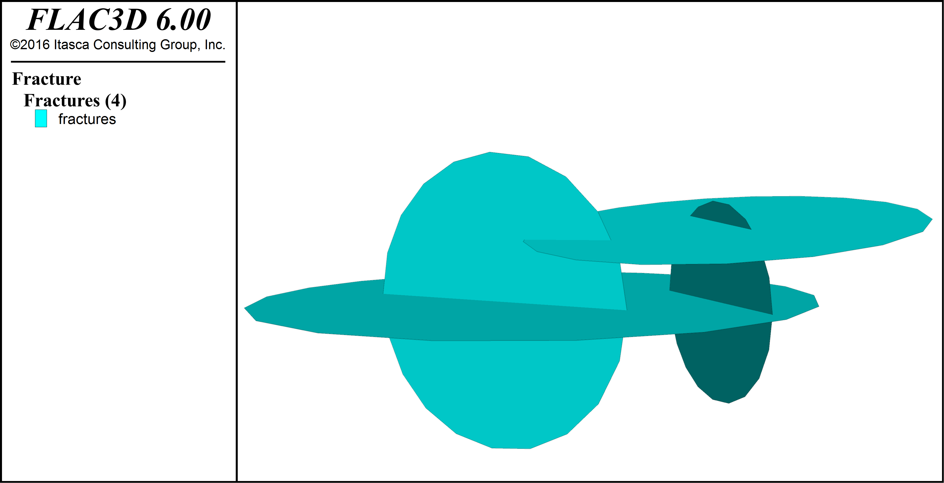
Figure 1: Deterministic fractures.
Intersections
An intersection object is the result of an intersection between a fracture and either a line,
a planar polygon, a convex set of planar polygons or another fracture. Intersection objects are modeled
by {a point in 2D; a segment or a collection of adjacent segments in 3D}. The figure below shows
the intersections, computed via the fracture intersections compute command, between the deterministic
fractures shown above. Fracture intersections are grouped into intersection sets for ease of processing.
For instance, one may determine the intersections between fractures and also the intersections between
fractures and a model of a borehole; these may be stored in separate intersection sets for later
processing.
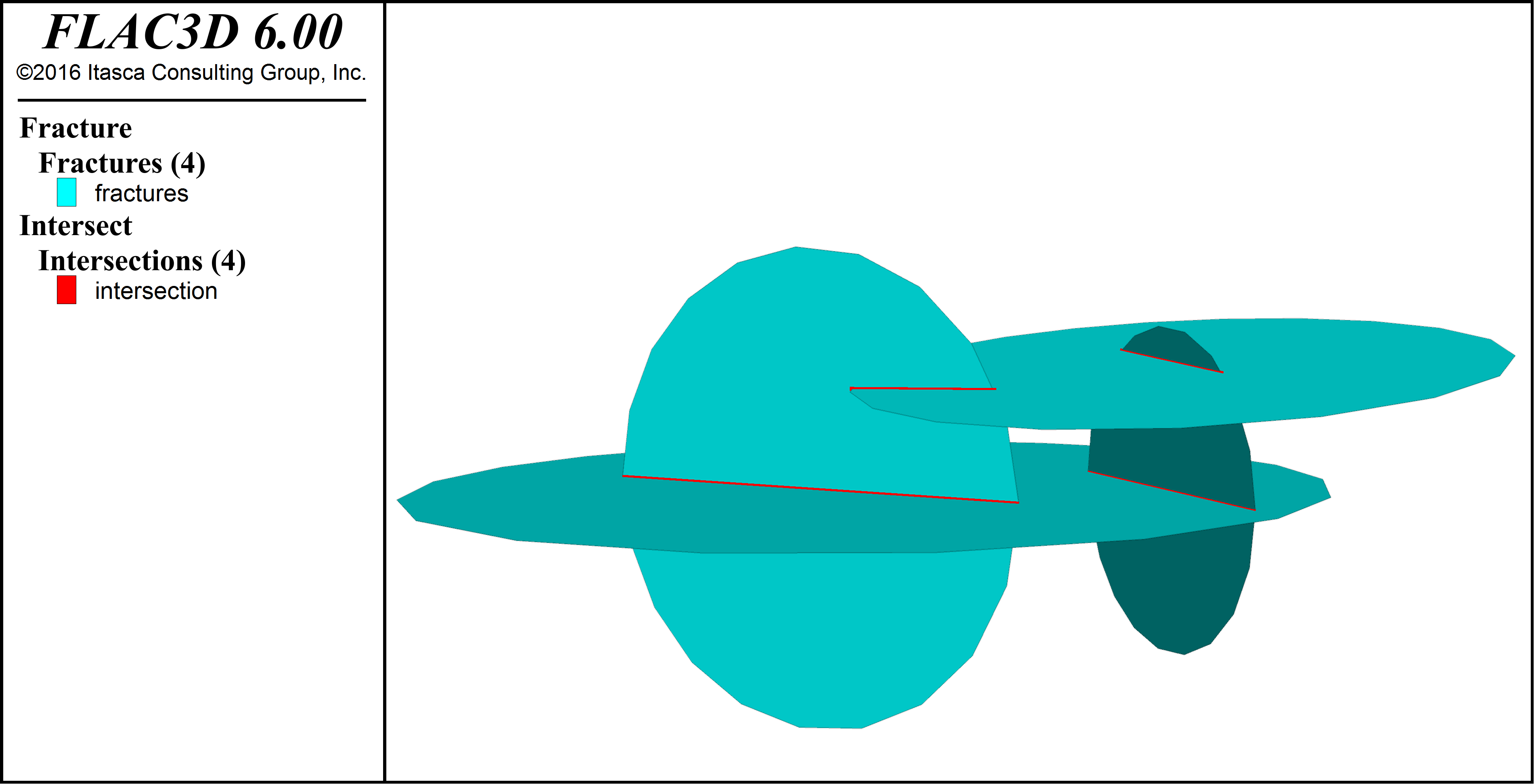
Figure 2: Intersections between deterministic fractures.
Generating Stochastic Fracture Sets or DFNs
A DFN is a set of fractures. In the figures above, there is a single DFN that is composed of four user specified fractures. Multiple DFNs, or sets of fractures, can exist simultaneously, though any fracture can only belong to a single DFN. The figure below shows two DFNs composed of deterministic fractures, one composed of horizontal fractures and one composed of vertical fractures. Splitting fractures into separate DFNs may be useful for computations involving different sets of fractures with different characteristics (i.e., in this example, horizontal versus vertical fracture sets). Stochastic fractures are generated in separate DFNs, as described below.
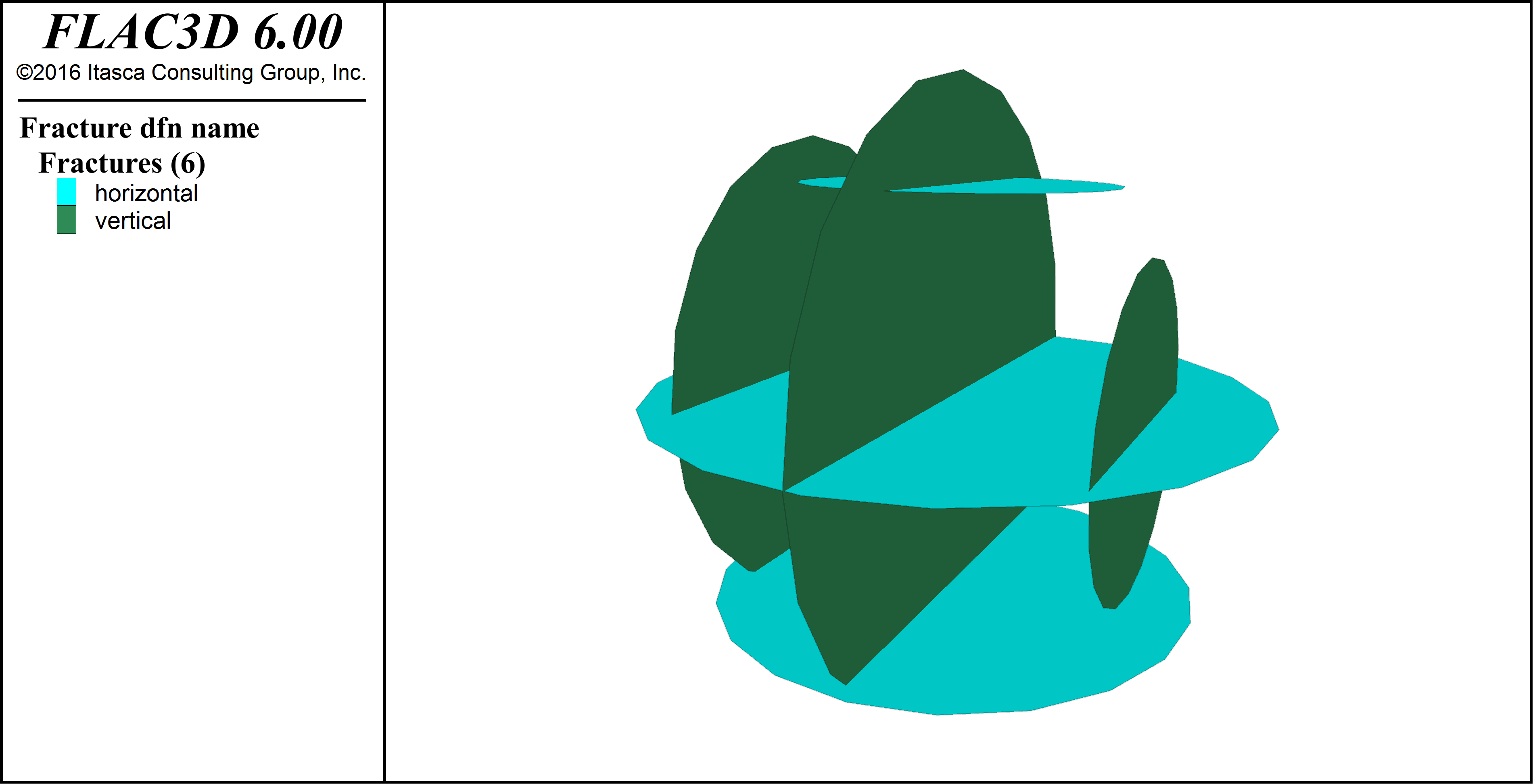
Figure 3: Two DFNs, or fracture sets, composed of horizontal and vertical fractures.
Stochastic Descriptions of Fractures - the Fracture Template
It is often the case that, in a rock mass, one cannot directly determine the sizes, orientations and
frequencies of the fractures pervading the rock mass. Instead, geological mapping and/or geophysical
techniques are used to estimate the characteristics of the fractures. After inspecting field data, one
may determine bounds on the fracture sizes, positions, and orientations. A fracture template holds
these statistical parameters and is used to generate stochastic fractures with the fracture generate
command. Specifically, the fracture template contains a description of the size, position and orientation
distributions of the fractures; it is created with the fracture template create command. Thus
a fracture template is a stochastic representation of a set of fractures and can be used to generate
any number of specific realizations of fractures.
Stochastic Modeling Approach
The modeling approach used to generate fractures is stochastic: the geometrical characteristics of fractures, usually obtained from field data, are constrained through independent statistical distributions (i.e., type of distribution and associated parameters) of their geometrical properties. This information is stored in a fracture template. The geometrical characteristics currently supported by fracture templates are the fracture size (diameter), orientation and position distribution. From one fracture template, any number of different realizations of fractures can be generated, depending on the random seed.
Fracture Size Density Distribution
The fracture size density distribution defines the number of fractures per unit of volume, \(n(l)\), whose size is in the range \([l; l+dl]\). It combines a fracture size probability distribution function and a density term. For a power law distribution, the relationship is
where \(a\) is the scaling exponent (since the power law exponent is always negative, equal to -\(a\), the scaling exponent is positive) and \(\alpha\) is the density term of the model. The distribution is between \(l_{min}\) and \(l_{max}\). These are the the lower and upper bounds of the fracture sizes, respectively. Note that since the distribution is not necessarily bounded toward its upper bound, \(l_{max}\) can be infinite. \(a\) precisely fixes, at any scale, the ratio between smaller and larger fracture sizes. Is it usually in the range \([3;4]\). When plotted on a log-log plot, \(n(l)\) appears as a straight line (see Figure 4) whose apparent slope is -\(a\).
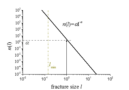
Figure 4: Power-law distribution in a log-log diagram.
The power law model encompasses end member models, such as the model of constant size \(l_{min}\) if \(a\rightarrow \infty\), or models with infinite fractures when \(a \leq 2\). When \(a\) increases, the proportion of small fractures increases relative to large fractures (Figure 5).
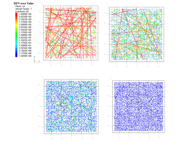
Figure 5: 2D outcrops from 3D DFNs generated within a cube of \(L=100\) with \(l_{min}=1\), \(l_{max}=100\) and \(d_m=1\) (see Table 1) with, from left to right and from top to bottom, \(a=2\), \(a=3\), \(a=4\) and \(a\rightarrow \infty\).
The term \(\alpha\) fixes the total fracture density by range of fracture size. The total fracture density (see below) is additionally dependent on the range of fracture sizes considered. The total number of fractures with sizes in the range \([l; l+dl]\), in a volume of characteristic size \(L\), is then defined as \(N(l,L)\) (e.g., \(N(l,L)=\alpha \cdot l^{-a}\cdot L^3\)).
If the domain is cubic, \(L\) is simply the side of the cube. The number of fractures with sizes between \(l_1\) and \(l_2\) is given by
The cumulative fracture size density distribution that defines the number of fractures whose size is larger than a given value \(C(l)\) is defined by
One sees that if the scaling exponent is large enough (e.g., \(\geq 4\)), a corresponding fracture population is dominated by the smallest fractures. In other words, \(l^{-a+1}\) decreases quickly with \(l\) if \(a\geq 4\). The power law model is not the only size distribution available in fracture templates. Gauss, uniform and bootstrapped (from file) distributions are also available. The user can also define a custom distribution with FISH.
Densities
The most common definition for the fracture density is related to the total surface (mass) of fracture per unit volume. In 3D, the fracture mass density is the total fracture surface area per unit volume (\(d_m\) or \(P_{32}\)). In 2D, it is the total fracture length per unit area (\(P_{21}\)). In 1D, it is the fracture frequency (\(f\) or \(P_{10}\)): the number of fracture intercepts by unit length of the scanline. The fracture density may also be defined as a fracture center density: the number of fracture centers per unit volume (\(d_c\) or \(P_{30}\)). These definitions are shown in Table 1. In order to simplify modeling with the DFN module, the required density (i.e., input of the fracture generation) is defined from either the mass density, center density or the fracture frequency, each of them relying on estimates from a sample. For any given initial density, the spatial distribution of fracture positions arises from a Poisson process, leading to a uniformity of fracture positions throughout the volume.
Name |
Unit |
Meaning |
Link to fracture size distribution |
|---|---|---|---|
mass density (\(dm\) or \(P_{32}\)) |
\(m^2/m^3\) |
Cumulated surface of fracture per unit volume |
\(d_m(l_c)\cong \int_{l_c}^\infty n(l)\cdot l^2\cdot L^{-3}\cdot dl\) |
mass density on outcrop (\(P_{21}\)) |
\(m/m^2\) |
Cumulated length of fracture per unit surface |
\(P_{21}(t_c)\cong \int_{t_c}^L n(t,L)\cdot\cdot L^{-2} dt\). \(t\) is the fracture trace line observed on a 2D outcrop. |
fracture frequency (\(f\) or \(P_{10}\)) |
\(m^{-1}\) |
Number (N) of fractures per unit length |
\(f(l_c)\propto K_{ori}\cdot d_m(lc)\). \(K_{ori}\) depends on the respective orientation of the 1D scanline or borehole and the DFN orientation distribution. In the case of uniform orientation (no preferential direction), \(K_{ori}=0.5\). |
center density (\(d_c\) or \(P_{30}\)) |
\(m^{-3}\) |
Number of fracture centers per unit volume |
\(d_c(l_0)=\int_{l_0}^L n(l)\cdot L^{-3}\cdot dl\) |
fracture spacing |
\(m\) |
Inverse of fracture frequency average distance between fractures along a 1D line |
\(\text{spacing}(l_c)=\frac{1}{f(l_c)}\) |
percolation parameter |
\(m^3/m^3\) |
Cumulated excluded volume around fractures per unit volume |
\(d_m(l_c)\cong \int_{l_c}^\infty n(l)\cdot l^3\cdot L^{-3}\cdot dl\) |
Fracture density is a scale-averaging property, meaning that fracture density estimates and associated distributions depend on the location and scale of the observation region. They can reflect local variability, when the observation scale tends to zero, or define bulk or macroscopic properties when the measurement scale tends to \(\infty\). The parameters \(a\), \(\alpha\), \(l_{min}\), \(l_{max}\), of the fracture size density distribution, fully define the fracture bulk density. However, field data of observed fracture densities are taken at finite size samples such as borehole sections, scanlines, or outcrop maps, and thus are related to their sample support. They potentially differ locally from the bulk fracture density. In addition, they are related to a limited range of fracture sizes, due to resolution effects at small sizes, and censoring and truncation at larger sizes.
| Was this helpful? ... | Itasca Software © 2024, Itasca | Updated: Dec 05, 2024 |
