FLAC3D Theory and Background • Constitutive Models
Curved Mohr-Coulomb Model
The traditional Mohr-Coulomb model assumes that a linear shear failure develops, which is just a simplification by linear extrapolation of the experimental data over a limited stress range. However, experimental data covering low stresses clearly show a curved failure envelope for a wide range of geomaterials from clay to rockfill. As such, this simplification could significantly overestimate safety factor, particularly for a shallow slip surface or near the excavated zones exhibiting low normal stress.
The linear Mohr-Coulomb model represents a shear failure criterion with a simple linear relationship between the shear strength \(\tau\) versus the applied normal stress \(\bar{\sigma}_n\) (positive in compression in this model if with a bar), which can be expressed by
(1)\[\tau = \bar{\sigma}_n \tan{\phi} + c\]
where \(c\) is often called the cohesion and the angle \(\phi\) is called the angle of internal friction. This shear failure criterion can be alternatively expressed by a linear relationship between the maximum and minimum principal stresses.
(2)\[\bar{\sigma}_1 = N_f \bar{\sigma}_3 + N_c\]
where \(\bar{\sigma}_1 = -\sigma_1\) and \(\bar{\sigma}_3 = -\sigma_3\), \(N_f = (1+\sin{\phi})/(1-\sin{\phi})\), \(N_c = 2c\sqrt{N_f}\).
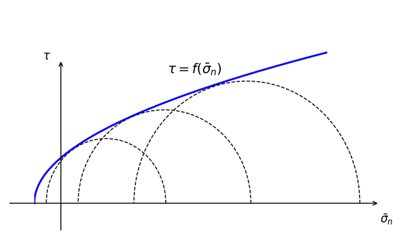
In many cases, the linear strength formulation of the Mohr-Coulomb model is just a simplification. The more general form is a curved strength with the form of \(\tau\) vs. \(\bar{\sigma}_n\) (see Figure 1):
(3)\[\tau = f(\bar{\sigma}_n)\]
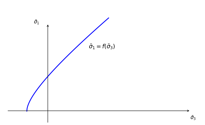
or as in the Hoek-Brown model, in a form of \(\bar{\sigma}_1\) vs. \(\bar{\sigma}_3\) (see Figure 2):
(4)\[\bar{\sigma}_1 = f(\bar{\sigma}_3)\]

Figure 1: Curved strength defined by \(\tau\) vs. \(\bar{\sigma}_n\).

Figure 2: Curved strength defined by \(\bar{\sigma}_1\) vs. \(\bar{\sigma}_3\).
Model description
Elasticity
In this model, the elastic moduli can have options being of constant or stress-dependent:
index-elasticity = 0 (default)
For this default case, the elastic moduli are assumed constants. We can input either bulk and shear moduli (\(K\) and \(G\)), or Young’s modulus and Poisson’s ratio (\(E\) and \(\nu\)).
index-elasticity = 1
where \(p\) is the current effective mean pressure, \(E_{ref}\) and \(n\), are material constants. \(p_{ref}\) is a reference pressure which should be consistent to the unit in the model. The lower-bound of the stress-depend Young’s modulus is \(E = 0.01E_{ref}\). For this case, Poisson’s ratio \(\nu\) is required as well.
Strength
The shear strength can be defined based on the input value of index-strength.
index-strength = 0
In this case, the curved strength is pre-defined by the power form
(6)\[\tau = b p_{ref} {\left( \frac{\bar{\sigma}_n}{p_{ref}} + s \right)}^a\]
where \(a\), \(b\) and \(s\) are material constants without any unit, and \(p_{ref}\) is the reference pressure. \(a\) is limited to the range between 0 and 1. The tension strength is the minimum between the input tension \(\sigma^t\) and \(s p_{ref}\).
when \(a\) = 1, it degrades to the linear Mohr-Coulomb model with the relationships \(b = \tan{\phi}\) and \(s = c/bp_{ref}\);
when \(a\) = 0, it degrades to the linear Mohr-Coulomb model with zero friction angle and with the relationships \(b = c/p_{ref}\).
index-strength = 1
In this case, the curved strength is pre-defined by the form
(7)\[\bar{\sigma}_1 = \bar{\sigma}_3 + p_{ref} \left(b \frac{\bar{\sigma}_3}{p_{ref}} + s \right)^a\]
where \(a\), \(b\) and \(s\) are material constants without any unit, and \(p_{ref}\) is the reference pressure. If \(p_{ref}\) is represented by the unconfined uniaxial strength, it is the same as the Hoek-Brown shear failure criteria. The tension strength is the minimum between the input tension \(\sigma^t\) and \(s p_{ref}/b\).
index-strength = 2
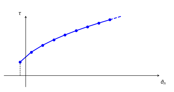
In this case, as shown in Figure 3, the curved strength is defined by a piecewise curve with pairs of (\(\tau\), \(\bar{\sigma}_n\)). These pairs can be input as a table-like property. The tension strength is the minimum between the input tension \(\sigma^t\) and the value of \(\bar{\sigma}_n\) in the first pair.
If defined by merely two pairs, it is the special case of linear Mohr-Coulomb model.
If defined by three pairs, it is the shear failure of the SUBI model.
If defined by many pairs on the curve of Equation (6), it can approximately fit with the power-form failure line.

Figure 3: Curved strength defined by piecewise pairs of (\(\tau\), \(\bar{\sigma}_n\)).
index-strength = 3
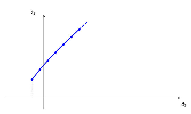
In this case, as shown in Figure 4, the curved strength is defined by a piecewise curve with pairs of (\(\bar{\sigma}_1\), \(\bar{\sigma}_3\)). These pairs can be input as a table-like property. The tension strength is the minimum between the input tension \(\sigma^t\) and the value of \(\bar{\sigma}_3\) in the first pair.
If defined by merely two pairs, it is the special case of linear Mohr-Coulomb model.
If defined by three pairs, it is the shear failure of the SUBI model.
If defined by many pairs on the curve of Equation (7), it can approximately fit with the Hoek-Brown shear failure line.

Figure 4: Curved strength defined by piecewise pairs of (\(\bar{\sigma}_1\), \(\bar{\sigma}_3\)).
Dilation
In this model, the dilation angle can be a fixed value or a fixed factor of the current equivalent friction angle.
index-dilation = 0
The dilation angle is a factor (dilation-factor)of the current friction angle, which is determined either from the tangent line of the curve or the slope of the current segment associated to the current stress.
index-dilation = 1
The dilation angle is a fixed value of the input, dilation.
FOS Calculation
The Curved Mohr-Coulomb constitutive model is available to use with the automatic factor of safety (FOS) calculation.
Property List
Category |
Names |
Default |
|---|---|---|
Elasticity |
index-elasticity (if = 0): |
0 |
bulk (\(K\)), shear (\(G\)), or |
||
young (\(E\)), poisson (\(\nu\)) |
||
index-elasticity (if = 1): |
||
young-reference (\(E_{ref}\)) |
||
exponent (\(n\)) |
0.0 |
|
pressure-reference (\(p_{ref}\)) |
||
pressure-effective (\(p\)) |
||
poisson (\(\nu\)) |
||
Shear Strength |
index-strength (if = 0 or 1): |
0 |
constant-a (\(a\)) |
||
constant-b (\(b\)) |
||
constant-s (\(s\)) |
0.0 |
|
pressure-reference (\(p_{ref}\)) |
||
index-strength (if = 2 or 3): |
||
table-strength |
||
Tension Strength |
tension (\(\sigma^t\)): |
0.0 |
Dilation |
index-dilation (if = 0): |
0 |
dilation-factor |
0.2 |
|
index-dilation (if = 1): |
||
dilation |
0.0 |
|
Read-Only |
cohesion (\(c\)) |
|
friction (\(\phi\)) |
Examples
Frequently Asked Questions
Q: Why is the input strength positive in compression?
A: The input strength is positive because the table defining the curved strength must be sorted monotonically for x-values.
Q: What happens if the stress in the model is out of the range of the piecewise curve?
A: If the stress is out of the range on the left side, it indicates tension failure, and the tension failure rule of the Mohr-Coulomb model applies. If the stress is out of the range on the right side, the last segment of the curve is assumed to extend beyond the defined range and the shear failure rule of the Mohr-Coulomb model applies.
Q: Are there any requirements for the input table defining the curved strength?
A: Yes, the table pairs must be monotonically increasing to ensure positive friction angle and cohesion for any segment.
Q: How is tension determined?
A: Tension \(\sigma^t\) is determined as the minimum of the input of tension (with a default of zero) and either the apex value (for index-strength = 0 or 1) or the absolute value of the minimum x-value of the input piecewise curve (for index-strength = 2 or 3). Note that tension cannot be a negative value so it is possible minimum value is zero for all cases. Specifically,
index-strength = 0, \(\sigma^t = min(\sigma^t, sp_{ref})\)
index-strength = 1, \(\sigma^t = min(\sigma^t, sp_{ref}/b)\)
index-strength = 2, \(\sigma^t = min(\sigma^t, -\bar{\sigma}_{n,1})\)
index-strength = 3, \(\sigma^t = min(\sigma^t, -\bar{\sigma}_{3,1}))\)
Q: How to use the apex value or the leftmost x-value as the tension?
A: Just input a very large value, for example, tension = 1e20, then the above rules will apply and ensue the expected tension as the apex value or the leftmost x-value.
mohr-coulomb Model Properties
Use the following keywords with the zone property (FLAC3D) or block zone property (3DEC) command to set these properties of the Curved-Mohr-Coulomb model.
- bulk f
elastic bulk modulus, \(K\)
- constant-a f
constant-a, \(a\). Required only when index-strength is 0 or 1.
- constant-b f
constant-b, \(b\). Required only when index-strength is 0 or 1.
- constant-s f
constant-s, \(s\). Required only when index-strength is 0 or 1.
- index-strength i
index of strength, the default is 0.
if set to 0, the curved strength is defined by the power formulation of \(\tau\) vs. \(\bar{\sigma}_n\);
if set to 1, the curved strength is defined by the Hoek-Brown formulation of \(\bar{\sigma}_1\) vs. \(\bar{\sigma}_3\);
if set to 2, the curved strength is defined by a table with pairs of (\(\tau\), \(\bar{\sigma}_n\));
if set to 3, the curved strength is defined by a table with pairs of (\(\bar{\sigma}_1\), \(\bar{\sigma}_3\)).
- poisson f
Poisson’s ratio, \(\nu\)
- pressure-reference f
reference pressure, \(p_{ref}\). Required only when index-strength is 0 or 1, or index-elasticity is 1.
- shear f
elastic shear modulus, \(G\)
- young f
Young’s modulus, \(E\)
- dilation f (a)
dilation angle, \(\psi\). Required when index-dilation = 1, with the default 0.0. It is read-only when index-dilation = 0.
- dilation-factor f (a)
dilation factor (default = 0.2), this is required when index-dilation is 0 (default) and the current dilation angle will be the current equivalent friction angle multiplied by this value. The current equivalent friction angle is calculated and related to the current tangle line of the curved strength.
- exponent f (a)
The exponent \(n\). Required only when index-elasticity is 1. the default is 0.
- flag-brittle b (a)
If true (or on or yes), the tension limit is set to 0 in the event of tensile failure. The default is false.
- index-dilation i (a)
index of dilation, the default is 0.
if set to 0, the dilation will be a factor (assigned by dilation-factor) of the current friction angle;
if set to 1, the dilation will be the value input by dilation.
- index-elasticity i (a)
index of elasticity, the default is 0.
if set to 0, the elastic modulus are assumed constants;
if set to 1, the elastic modulus are stress-dependent.
- pressure-effective f (a)
Effective mean pressure, \(p\). Required to be assigned the first time this model is initialized when index-strength is 1. it will be updated during calculation.
- table-strength s (a)
name of the table relating to piece-wised curved strength. Required only when index-strength is 2 or 3.
- young-reference fa
Reference Young’s modulus, \(E_{ref}\). Required only when index-elasticity is 1.
- cohesion f (r)
current equivalent cohesion, \(c\)
- friction f (r)
current equivalent friction angle, \(\phi\)
Key
- (a) Advanced property.
This property has a default value; simpler applications of the model do not need to provide a value for it.
- (r) Read-only property.
This property cannot be set by the user. Instead, it can be listed, plotted, or accessed through FISH.
- Notes
Only one of the two options is required to define the elasticity: bulk modulus \(K\) and shear modulus \(G\), or Young’s modulus \(E\) and Poisson’s ratio \(\nu\). When choosing the latter, Young’s modulus \(E\) must be assigned in advance of Poisson’s ratio \(\nu\).
| Was this helpful? ... | Itasca Software © 2024, Itasca | Updated: Dec 05, 2024 |
