Axially Loaded Pile: Skin Friction

Problem Statement

Note

The project file for this example is available to be viewed/run in FLAC2D. The main data files used are shown at the end of this example. The remaining data files can be found in the project.

Piles transfer axial loads to the ground via two mechanisms: skin friction and end bearing. Both are examined in the following examples.

Engineering solutions for axially loaded piles are commonly based on axisymmetric point-load solutions (e.g. the Boussinesq solution - see [Geddes1969]). In FLAC2D, the pile is represented in plane-strain as a pile wall extending out the plane of the cross section. In the following examples the engineering solution is adapted to the plane-strain formulation. Although piles in FLAC2D cannot be applied to simulate a single pile, the plane-strain formulation can be used to represent equally spaced piles.

Skin Friction - In this example, the vertical stress in the ground (calculated by FLAC2D) that results from uniform skin friction resistance of an axially loaded pile, are compared to those estimated from a simple stress approximation. The approximation is based on integration of the Flamant solution for a point load on an elastic half-plane (adapted from the [Terzaghi1943] and [Geddes1969] approach to the plane-strain case).

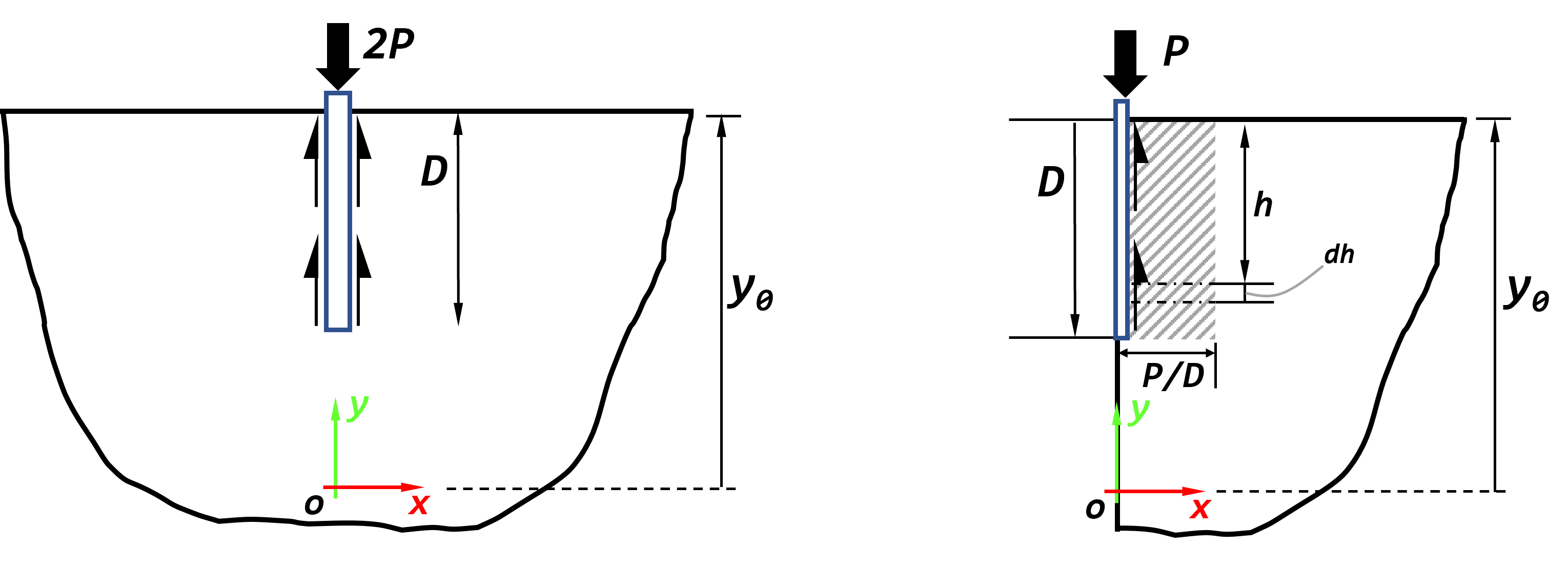
A total axial load $2P$ is applied at the top of a vertical pile of length $D$. A system of Cartesian axes is defined with the y-axis pointing upwards along the pile, and the pile top is at elevation $y_0$ (see Figure 1).

../../../../../_images/skinfriction.png — Figure 1: Friction pile loading conditions.

The load is transferred to the medium through uniform skin friction by selecting a constant shear spring stiffness, $k_s$, that is two orders of magnitude smaller than both the medium bulk modulus, $K$, and the pile axial stiffness, $E$. The shear cohesion, $c_s$, is set to a high value to prevent shear yielding.

For comparison to the stress-approximation solution, far-field stress boundary conditions, that correspond to the Flamant solution for a point surface load of intensity $2P$ are applied. This solution has the form,

(1)\[\begin{split}\sigma_{xx} = {{-4P} \over {\pi}} {{(y_0 - y)x^2} \over {[(y_0 - y)^2 + x^2]^2}} \\ \sigma_{yy} = {{-4P} \over {\pi}} {{(y_0 - y)^3} \over {[(y_0 - y)^2 + x^2]^2}} \\ \sigma_{xy} = {{4P} \over {\pi}} {{(y_0 - y)^2x} \over {[(y_0 - y)^2 + x^2]^2}}\end{split}\]

In the stress-approximation solutions, the stresses due to uniform skin friction are estimated by assuming a load distribution of intensity $P/D$ over a vertical height $D$ (see Figure Figure #axiallyloaded-pile2d1). Neglecting the influence of the overburden ar the elevation $y = y_0 - h$, and using the Flamant solution, the vertical stress contribution caused by a load increment $dP/dh = P/D$ over the height $dh$ may be approximated by

(2)\[d\sigma_{yy} = {{-2P} \over {{\pi}D}} {{(y_0 - h - y)^3} \over {[(y_0 - h - y)^2 + x^2]^2}}\]

Summing up incremental load contributions above the current elevation, we obtain,

(3)\[ \begin{align}\begin{aligned}\begin{split} \quad \sigma_{yy} = {{-2P} \over {{\pi}D}} \int_0^a {{(y_0 - h - y)^3} \over {[(y_0 - h - y)^2 + x^2]^2}} \,dh \\ \\\end{split}\\\begin{split} \mbox{with }\quad a = \left\{ \begin{array}{rl} y_0 - y, & \mbox{$y \ge y_0 - D$} \\ D , & \mbox{$y \le y_0 - D$} \end{array} \right.\end{split}\end{aligned}\end{align} \]

Upon integration, we obtain, for $y \ge y_0 - D$,

(4)\[\sigma_{yy} = {{P} \over {{\pi}D}} \biggl[ ln{{x^2} \over {(y_0 - y)^2 + x^2}} + {{(y_0 - y)^2} \over {(y_0 - y)^2 + x^2}} \biggr]\]

and, for $y \le y_0 - D$,

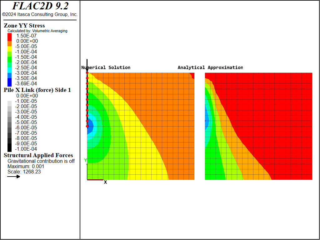
(5)\[\small {\sigma_{yy} = {{P} \over {{\pi}D}} \biggl[ ln{{(y_0 - D - y)^2} \over {(y_0 - y)^2 + x^2}} + {{x^2} \over {(y_0 - D - y)^2 + x^2}} - {{x^2} \over {(y_0 -y)^2 + x^2}} \biggr]}\]

Vertical stresses calculated by FLAC2D are compared to those given in Equation (4) and (5).

Note that combined damping, rather than local damping, is used for this example (see Damping Formulation for a discussion on damping modes).

Figure 2 shows contours of vertical stress obtained numerically (left) and the analytical approximation (right). The same order of magnitude for the stresses is obtained in the two solutions. Discrepencies between the two responses may be attributed to the approximate character of the analytical solution. This example serves to demonstrate the capability of FLAC2D to transmit loads adequately to the medium by means of the coupling-spring connections.

../../../../../_images/verticalstress.png — Figure 2: Shear force at the pile-grid boundary and verticat stress for *FLAC2D* (Left) and the analytical approximation (Right).

References

[Geddes1969] (1,2)

Geddes, J.D. “Boussinesq-Based Approximations to the Vertical Stresses Caused by Pile-Type Subsurface Loadings”, in Geotechnique Vol. 19(4), pp. 509-514, 1969.

[Terzaghi1943]

Terzaghi, K. “Theoretical Soil Mechanics”, London: Chapman and Hall, 1943.

Data File

SkinFriction.dat

; Axially loaded pile with skin friction example application
model new
model large-strain off
model title "Axially Loaded Pile: Skin Friction (2D)"

; Create the grid
[global top_ = 10]
zone create quadrilateral point 0 (0,0) point 1 (10,0) point 2 (0,[top_]) point 3 (10,[top_]) size 20 20
; Assign constitutive model and properties
zone cmodel assign elastic
zone property bulk=5e2 shear=3e2 density=2000

[global appliedLoad_ = -1e-3] ; Load applied at surface point and pile top
[global piledepth_ = 5] ; pile depth

; specify boundary conidition for symmetry plane
zone gridpoint fix velocity-x range position-x 0

; Far field boundary conditions (according to Flamant solution)
fish define FlamantStressNormal(zp,face)
  local x_ = zone.pos(zp)->x
  local y_ = zone.pos(zp)->y
  if (face = 3)
    FlamantStressNormal = ((top_ - y_)^3)/(((top_ - y_)^2 + x_^2)^2)
  else if (face = 2)
    FlamantStressNormal = ((top_ - y_)*x_^2)/(((top_ - y_)^2 + x_^2)^2)
  endif
end

fish define FlamantStressXY(zp)
  local x_ = zone.pos.x(zp)
  local y_ = zone.pos.y(zp)
  FlamantStressXY = ((top_ - y_)^2*x_)/(((top_ - y_)^2 + x_^2)^2)
end

zone face apply stress-yy [4*appliedLoad_/math.pi] fish-local FlamantStressNormal range position-y 0.0
zone face apply stress-xy [-4*appliedLoad_/math.pi] fish-local FlamantStressXY range position-y 0.0

zone face apply stress-xx [4*appliedLoad_/math.pi] fish-local FlamantStressNormal range position-x 10.0
zone face apply stress-xy [-4*appliedLoad_/math.pi] fish-local FlamantStressXY range position-x 10.0

zone gridpoint fix velocity-y range position (0,0)

; create the pile
structure pile create by-line (0,10) (0,[piledepth_]) segments 10
structure pile property young 5e2 cross-sectional-area 0.5 moi 0 ...
                        coupling-stiffness-shear 1 ... ; soft spring
                        coupling-cohesion-shear 1e10 ...
                        coupling-stiffness-normal 0 ...
                        perimeter 1

structure node apply force (0,[appliedLoad_]) range group 'Pile Begin'
structure mechanical damping combined-local

model history mechanical convergence
zone history displacement-y position (0,[top_])
zone history velocity-y position (0,[top_])
model solve convergence 1

model save 'SkinFriction'

AnalyticalApproximation.dat

model restore 'SkinFriction.sav'

fish define AnalyticalSolZoneExtra
  loop foreach local zp zone.list()
    local x_ = zone.pos.x(zp)
    local y_ = zone.pos.y(zp)
    if(y_ >= top_ - piledepth_)
      zone.extra(zp,1) = (-appliedLoad_/(math.pi*piledepth_))*(math.ln(x_^2/((top_-y_)^2 + x_^2)) + ... 
                         (top_-y_)^2/((top_-y_)^2 + x_^2))
    endif
    if(y_ <= top_ - piledepth_)
      zone.extra(zp,1) = (-appliedLoad_/(math.pi*piledepth_))*(math.ln(((top_-piledepth_-y_) + ... 
                         x_^2)/((top_-y_)^2 + x_^2)) + (x_^2/((top_-piledepth_-y_)^2 + x_^2)) - ...
                         (x_^2/((top_-y_)^2 + x_^2)))
    endif
  endloop
end
[AnalyticalSolZoneExtra]

model save 'AnalyticalApproximation'

⇄

⇐ Laterally Loaded Pile | Axially Loaded Pile: End Bearing ⇒

Was this helpful? ...

Updated: Dec 19, 2024