Tailing Dam Static Liquefaction (FLAC3D)

Problem Statement

Note

The project file for this example is available to be viewed/run in FLAC3D.[1] The project’s main data files are shown at the end of this example.

This example demonstrates the analysis of static liquefaction potential due to the construction of an additional layer (simplified by applying a surcharge). Key analysis procedures illustrated in this example include the following.

• Automatic grid generation by controlling zone size through the import of a soil profile geometry file.

• Staged construction simulation.

• Phreatic surface (water table) calculation.

• Static liquefaction analysis.

The model includes three basic materials: the starter dam, dikes, and tailings. The profile is shown in Figure 1.

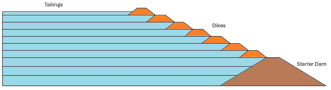
Figure 1: Model geometry of the tailing dam.

Modeling Procedure

Grid Generation

The model geometry is based on a DXF file named “tailingsdam-geometry.dxf”. The model is created interactively using the Sketch workspace. The State Record tab in the i Commands Area was used to convert the result to a data file called “sketch.dat”. The contents of the sketch set in the Sketch workspace can be be viewed after restoring any of the resulting data files.

The specific steps are as follows.

• After creating the project file, open the “File” menu, select “New”, then “Sketch Set”, and input a set name “tailings”. A sketch set called “tailings” will be created in the Sketch workspace.

• In the “tailings” set, click the “Import background image” button, then select the file “tailingsdam-geometry.dxf”. The geometry with nodes, edges, and polygons will be displayed in the Sketch workspace.

Once the background image is loaded into the workspace, automatically create edges from this image.

• Click the “Automatically create edges from background geometry” button.

• Click the “Mesh Tools” button, select “Auto-size”, and set the zoning using “zone length” with an input value of “1.0”.

• Click the “Mesh Tools” button again and select “Mesh All Polygons”.

At this point, the grid is automatically created with an approximate zone size of 1.0, which will be replaced by a FISH variable later. Next, assign group names to the sketch blocks and edges.

• Click the “Selection tool” button, click the sketch block of the starter dam, and input the group name “StarterDam” in the “Object Properties”.

• Similarly, input group names “Dike1” to “Dike7” for the sketch blocks of the dikes; input group names “Tailings01” to “Tailings10” for the sketch blocks of the tailings.

• Click the sketch edge of the uppermost tailing and input the group name “Load”.

After assigning group names to some sketch blocks and edges, proceed with the extrusion steps.

• Click “Bottom” view in the Sketch pane.

• Click the right point of the middle line. In the “Object Properties”, modify the Position’s W-coordinate to 1.

• Zoom in on the sketch, click or select the middle line. In the “Object Properties”, modify the “Zone number” to 1 and “Zone length” to 1.

• Click the “Create zones” button, the grid as shown in Figure 2 is created.

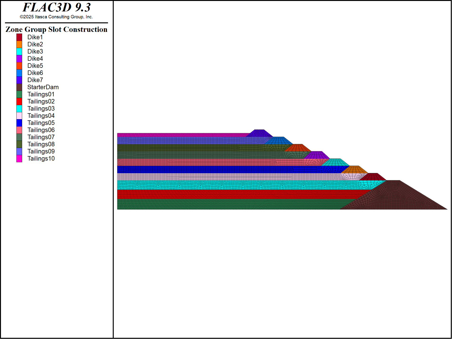
Figure 2: Soil Profile of the tailing dam.

All of the above operations in the Sketch workspace are recorded in the State Record tab in the i Commands Area. It is good practice to save these records into a data file so that later modifications can be made directly to the data file.

• Click the “State Record” tab. Right-click anywhere in the “State Record” window.

• Select “Save to file as datafile” and input a data file name, e.g., “sketch.dat”.

To ensure the sketch operations can be duplicated, follow these steps:

• Open the newly created data file and add the line “model new” at the very beginning.

• Run the data file; the sketch operations should be replicated.

• Add a line at the end to save the model, e.g., model save ‘sketch’.

If zone size adjustment is needed, a global FISH variable is assigned in the main data file. The corresponding values are modified into this FISH variable as follows.

• In the main data file, master.dat, input the first three lines as follows:

model new
[global zone_size = 1.0]
program call "sketch.dat"

• Comment out the first line (model new) in sketch.dat in case it has not been commented out. Otherwise, the FISH variable in the main data file cannot be transferred to sketch.dat.

• Modify the zone size in the corresponding lines of sketch.dat to use the assigned FISH variable.

; model new
...
sketch set automatic-zone direction construction edge [zone_size]
...
sketch segment-node id 2 move-to (75,30.25,[zone_size]) tolerance-merge 1
...
model save 'sketch'

Following these steps easily refines or coarsens the grid by simply adjusting the zone size variable in the main data file and re-running the script. This approach allows for quick and flexible modifications to the model’s resolution.

Staged Construction

This simulation is scripted in the datafile construction.dat.

After restoring the previous save file of grid generation, the command

zone face skin

is used to automatically assign face groups to the skins of the model. The face groups can be checked by plotting “zone->Face”. These face groups will be used later.

The model then sets some global configurations, including “fluid-flow”, “large-strain”, and “gravity” using the following commands.

model configure fluid-flow
model large-strain off
model gravity 9.81

The boundary conditions are simply the standard static boundary conditions.

zone face apply velocity-x 0 range group 'west' ;or 'east' 
zone face apply velocity-y 0 range group 'south' or 'north'
zone face apply velocity (0,0,0) range group 'bottom'

Because staged construction is to be simulated, all zones are first nulled using the command

zone null

The staged construction is simulated by reassigning the nulled zones to non-null materials. In this example, for simplicity, all materials are assumed to follow the Mohr-Coulomb model during the construction.

The starter dam is constructed first by assigning the “StarterDam” group to the Mohr-Coulomb model and setting the material properties. The command zone initialize-stresses is used to initialize the vertical stress to be gravitational and the horizontal stress to be a factor of the vertical stress. Use the command model solve-static convergence 1 to cycle through each staged construction.

zone cmodel assign mohr-coulomb range group 'StarterDam'
zone property density 2.0 bulk 3e5 shear 2e5 range group 'StarterDam'
zone property cohesion 20 friction 36 tension 1e20 range group 'StarterDam'
zone initialize-stresses ratio 0.6 range group 'StarterDam'
;
model solve-static convergence 1

After the construction of the starter dam, the displacement contour is shown in Figure 3.

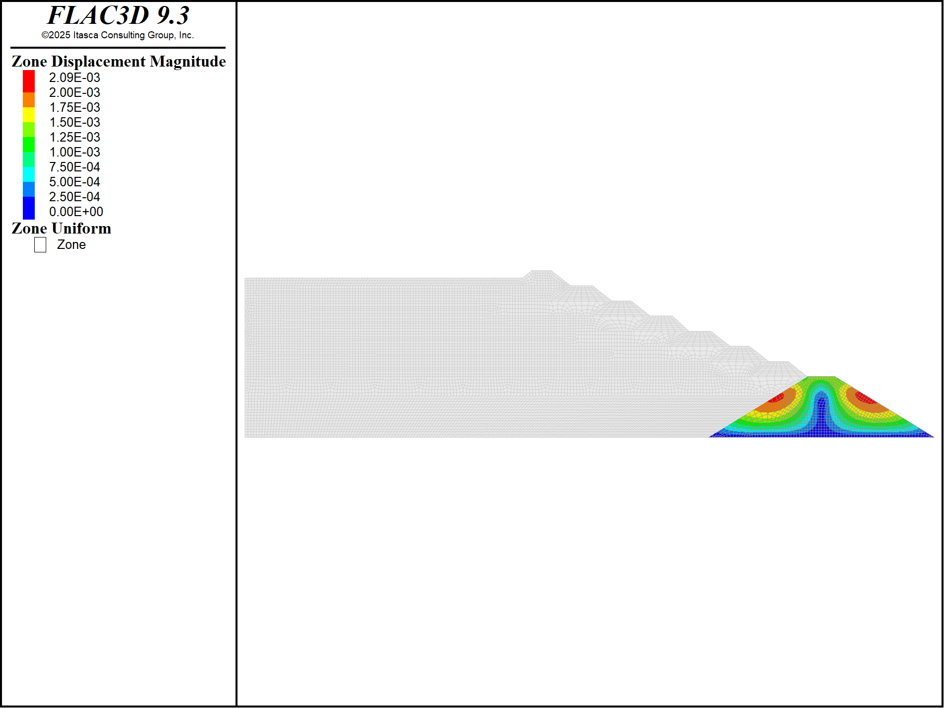
Figure 3: Displacement contour after construction of the starter dam.

For tailings and dikes, similar procedures can be adopted. Alternatively, a FISH function called “add_layer” is used for this purpose. The construction sequence is “StarterDam”, “Talings01”, “Talings02”, “Talings03”, “Dike1”, “Taings04”, “Dike2”, “Tailing05”, “Dike3”, “Tailing06”, “Dike4”, “Tailing07”, “Dike5”, “Tailing08”, “Dike6”, “Tailings09”, “Dike7”, and “Tailings10”. For example, Figure 4 shows the displacement contour after construction of Dike3.

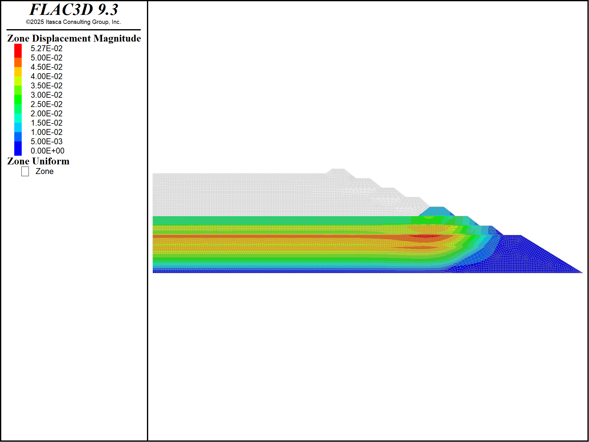
Figure 4: Displacement contour after construction of Dike3.

After completion of construction, the displacement contour is shown in Figure 5.

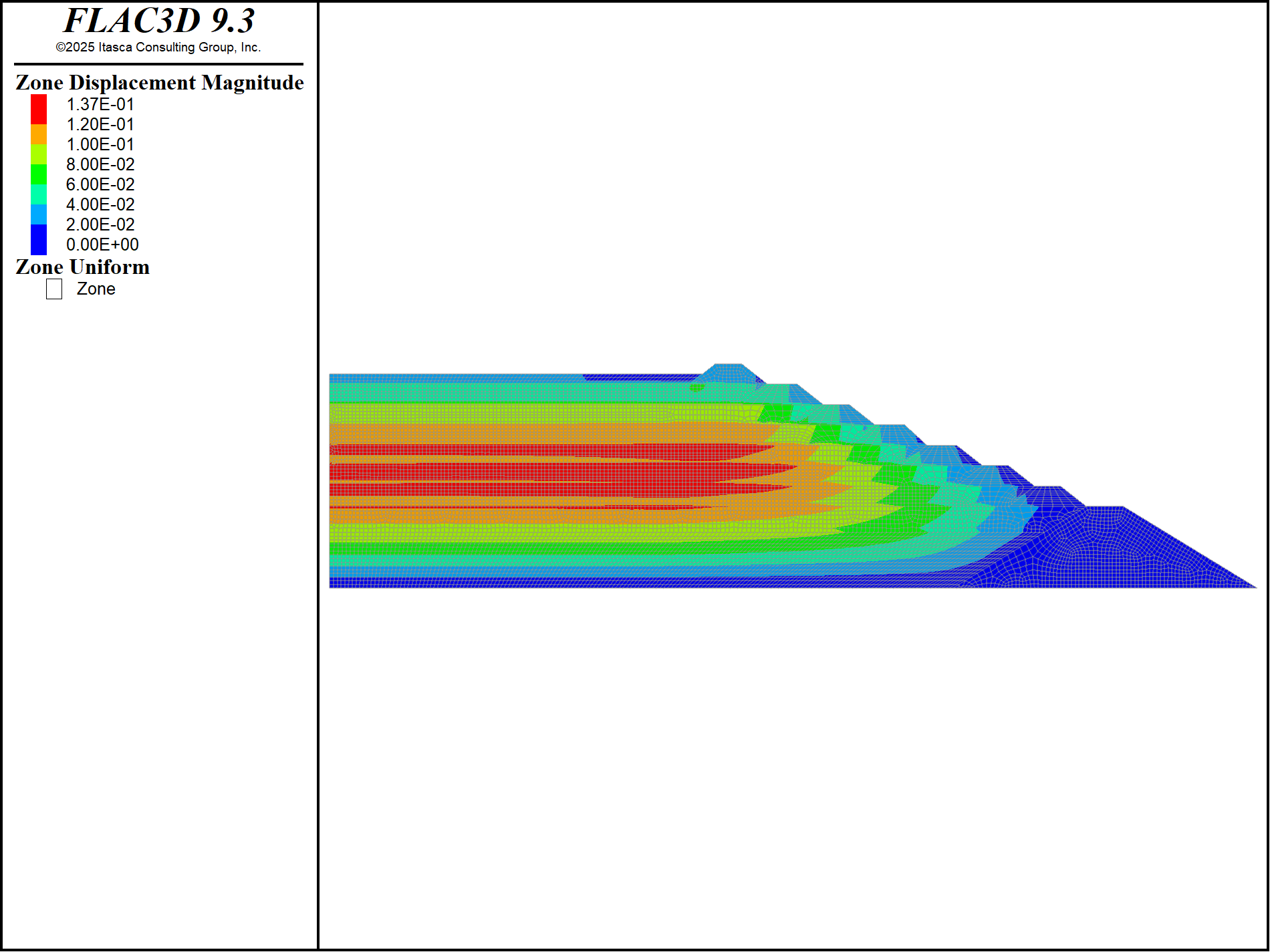
Figure 5: Displacement contour after construction completion.

Phreatic Surface Calculation

So far, no fluid has been considered. The stable phreatic surface needs to be calculated. This simulation is scripted in the data file fluid.dat.

After restoring the previous save file of the construction, the zone displacement, velocity, and plastic state are all re-initialized using the following commands.

zone gridpoint initialize velocity (0,0,0)
zone gridpoint initialize displacement (0,0,0)
zone initialize state 0

Fluid properties must now be input, such as “porosity,” “hydraulic-conductivity,” and fluid density. Note that “hydraulic-conductivity” here refers to Darcy’s coefficient, measured in units of [length/time]. It is different from another fluid property called “mobility-coefficient”, which is the value of “hydraulic-conductivity” divided by the fluid’s unit weight.

zone fluid property porosity 0.3 hydraulic-conductivity 1e-9
zone fluid-density 1

The saturation is initialized to be zero, and the saturation model is set to “cutoff” with the default cutoff value of zero.

zone gridpoint initialize saturation 0
; satuation model is set to cutoff 
zone fluid unsaturated cutoff

The fluid boundary conditions assume a fixed water table at the ground level on the “west” side and zero pore pressure at the top surface. Because the model base is at zero elevation (datum = 0), hydraulic head of 57.75 m is applied on the “west” side.

zone face apply head 57.75 range group 'west'
zone face apply pore-pressure 0 range group 'top'

To calculate a steady-state fluid solution, use the command:

zone fluid steady-state

With an unsaturated flow model present, the nonlinear effects are handled via Picard iteration. Because there is no transient response, it is not necessary to specify a fluid modulus (or Biot modulus) in the model. This command does not specify “effective on,” which means the default “effective off” is used — the solution will update the pore pressures but not the total stresses in the zones, resulting in a change of effective stress. The saturation contour and pore-pressure contour at the steady-state fluid solution are presented in Figure 6 and Figure 7, respectively.

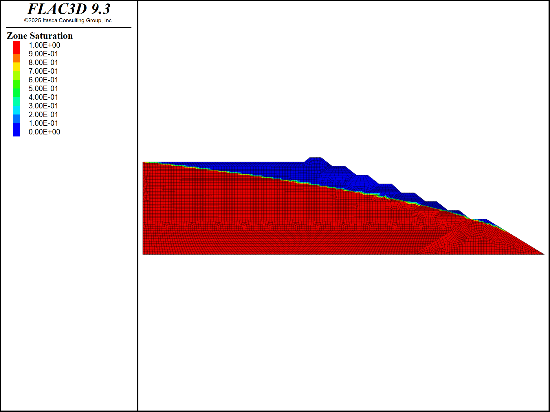
Figure 6: Saturation contour at the steady-state fluid solution.

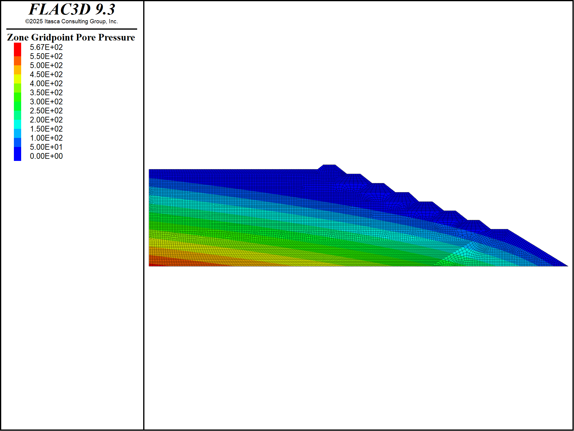
Figure 7: Pore-pressure contour at the steady-state fluid solution.

The above command is for fluid calculation only. A mechanical-only solution is required to cycle the model to mechanical equilibrium.

model solve-static convergence 1

Static Liquefaction

The model has completed staged construction, steady-state fluid calculation, and mechanical equilibrium. To analyze the potential for static liquefaction, the Mohr-Coulomb model for tailings is not sufficient because it does not incorporate the state parameter and thus cannot distinguish between dilative and contractive behaviors using one set of material constants. In this model, NorSand is used for tailings. This is implemented in the data file “toNorSand.dat” (see Figure 8).

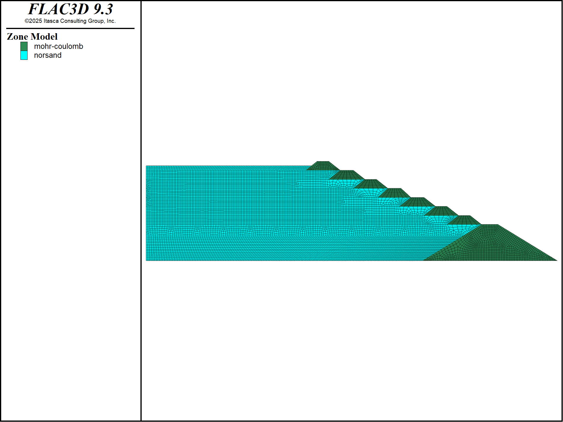
Figure 8: NorSand model for tailings and Mohr-Coulomb model for starter dam and dikes.

After the tailings have been changed to the NorSand model, the NorSand properties need to be input. The NorSand properties for tailings are summarized in Table 1.

Table 1: NorSand Properties for Tailings

Property	Symbol	Value
shear-reference	$G_{ref}$	2e4
exponent	$m$	0.72
pressure-reference	$p_{ref}$	100
poisson	$\nu$	0.15
critical-state-1	$C_1$	0.74
critical-state-2	$C_2$	0.05
critical-state-3	$C_3$	0.0
ratio-critical	$M_{tc}$	1.2
factor-dilatancy	$\chi_{tc}$	7.2
factor-coupling	$N$	0.25
hardening-0	$H_0$	45
hardening-y	$H_y$	30
flag-inner		on

In this example, the property “flag-inner” is turned “on” so that the inner cap yielding is considered. Note that the property “state-parameter-initial” (or “void-initial”) is significant to the material behavior. Refer to the documentation of the NorSand model for more details. In this model, for demonstration purposes, all tailings are set with an initial state parameter of 0.1, except for the first two tailing layers (“Tailings01” and “Tailing02”), which are set to -0.1 (Figure 8).

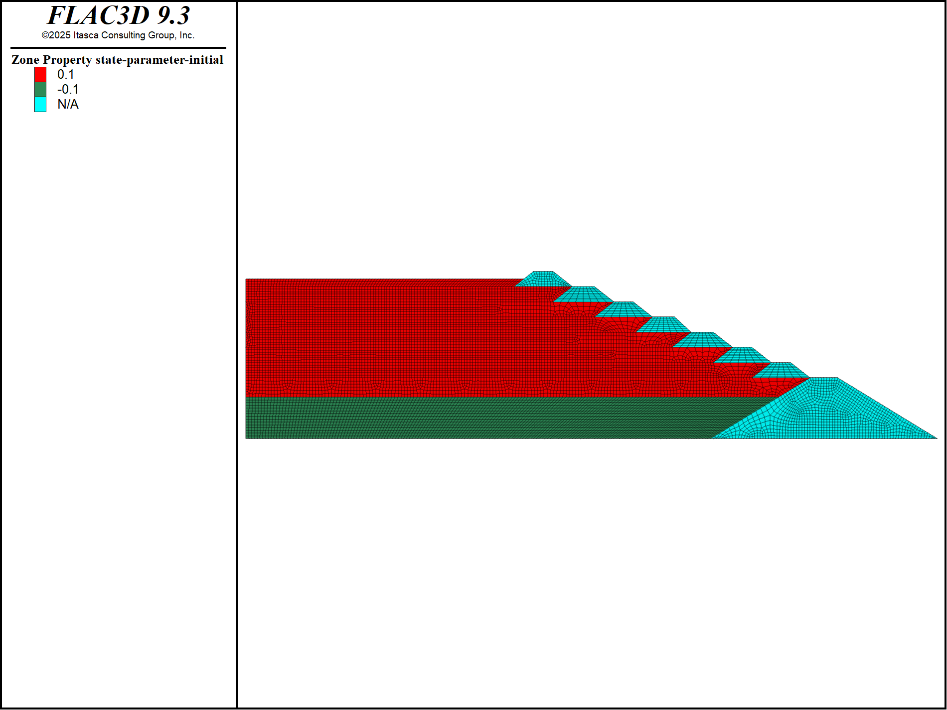
Figure 9: Initial state parameters of NorSand for tailings.

The NorSand model is stress-dependent because the moduli are a function of the current stress state. The previously calculated stress state is transferred to NorSand when the model is first assigned by a FISH function called “ini_stress.” This function uses the keyword “operator” instead of “define” and includes an argument for a specific zone (“zp”) that allows the function to be run multithreaded. Another argument (“modelName”) is included to designate the specific constitutive model.

fish operator ini_stress(modelName,zp)
  if zone.model(zp) = modelName then
    zone.prop(zp,'stress-xx-initial') = zone.stress.eff(zp)->xx
    zone.prop(zp,'stress-yy-initial') = zone.stress.eff(zp)->yy
    zone.prop(zp,'stress-zz-initial') = zone.stress.eff(zp)->zz
    zone.prop(zp,'stress-xy-initial') = zone.stress.eff(zp)->xy
    zone.prop(zp,'stress-yz-initial') = zone.stress.eff(zp)->yz
    zone.prop(zp,'stress-xz-initial') = zone.stress.eff(zp)->xz
  endif
end
[ini_stress("norsand", ::zone.list)]

After the NorSand model and properties for tailings are assigned, run the model to reach mechanical equilibrium.

The next analysis step (as in the datafile “static.dat”) is to evaluate the tailing dam’s potential for static liquidation due to a relatively quick surcharge on the current tailing surface. A surcharge might occur from additional tailing construction upon the current tailing surface.

First, reinitialize the zone displacement, velocity, and plastic state. Second, change the model to a relatively “undrained” condition. This requires two steps,

1. turn the pore-pressure generation to “on” with the command

zone fluid property pore-pressure-generation on

2. set the water bulk modulus to a non-zero value

zone fluid property fluid-modulus 2e5

Since the water is not confined on all boundaries, a compromised (reduced) water bulk modulus of 2e5 kPa is set, which is 1/10 of the real water bulk modulus of 2e6 kPa under perfectly confined conditions.

In this model, a “ramp” FISH function is used to gradually add the surcharge. This ramp function increases linearly from 0 to 1 in 6000 cycles steps and remains 1 thereafter.

[global iniStep = mech.step]
fish define ramp
  global cycles = mech.step - iniStep
  if cycles < 6000
    ramp = float(cycles)/float(6000)
  else
    ramp = 1.0
  endif
end

The surcharge is applied using the zone face apply stress-normal command, followed by a value of -500 multiplied by the ramp function, and applied to the face group “Load,” which is assigned in the data file sketch.dat.

; Apply surcharge
zone face apply stress-normal -500 fish ramp range group 'Load'

The model is cycled to 12000 steps. Figure 10 presents the shear band by plotting the contour of maximum shear strain increment. Figure 11 plots the contour of displacement. Both figures clearly demonstrate sliding failure due to static liquefaction. The displacement history at the highest dike top with coordinates (61,0,60.5) is plotted in Figure 12, which shows an accelerating increase, indicating an unstable slope.

The stress paths of selected zones (see gold dots in Figure 10), as well as the critical state line in the $q$ vs $p'$ plane are plotted in Figure 13. All these selected zones are located within the shear bands, and their final shear strengths are lower than their initial strengths, which are clear indicators of static liquefaction.

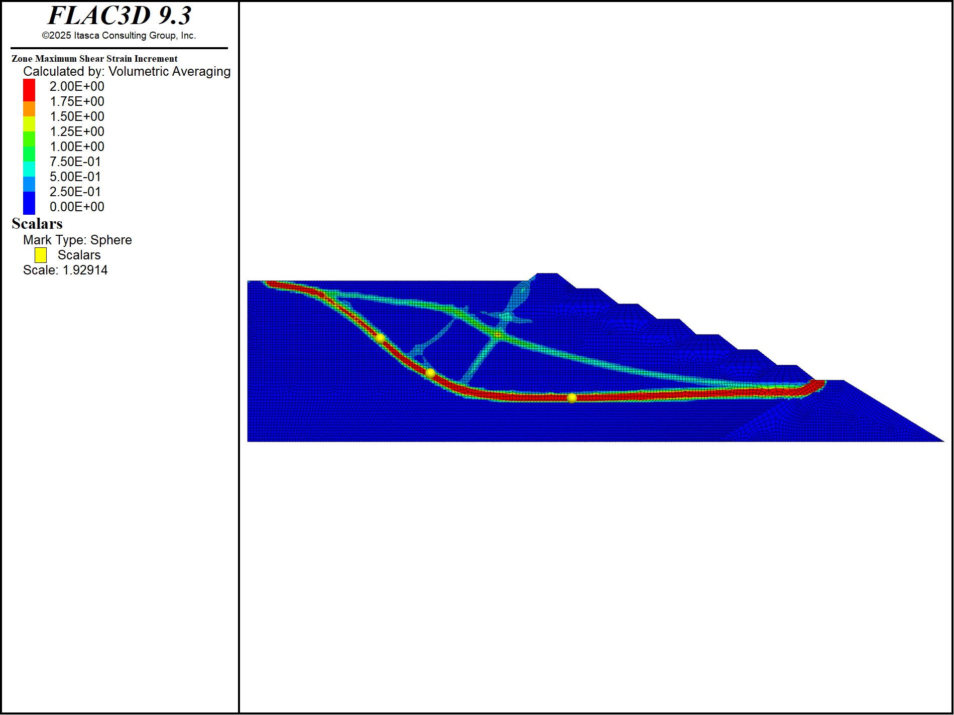
Figure 10: Maximum shear strain contour indicating localized shear bands induced by static liquefaction.

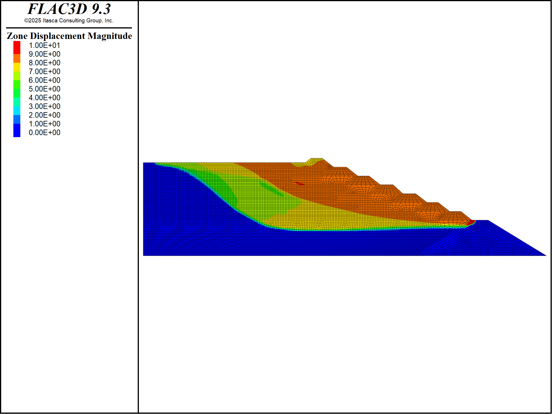
Figure 11: Displacement contour indicating sliding failure induced by static liquefaction.

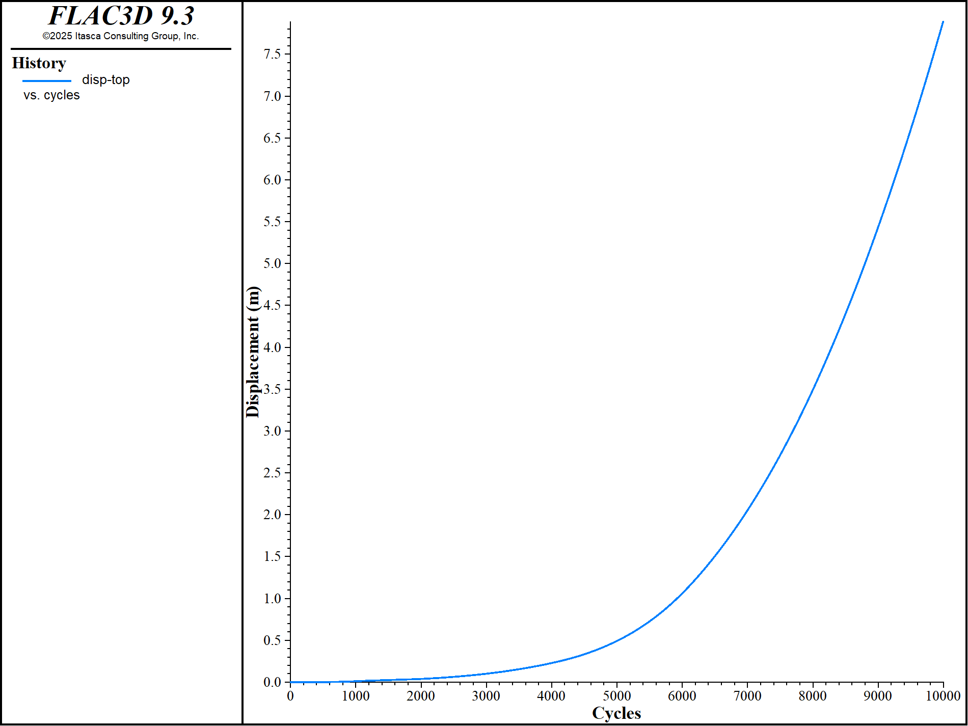
Figure 12: Displacement history at the highest dike top with coordinates (61,0,60.5).

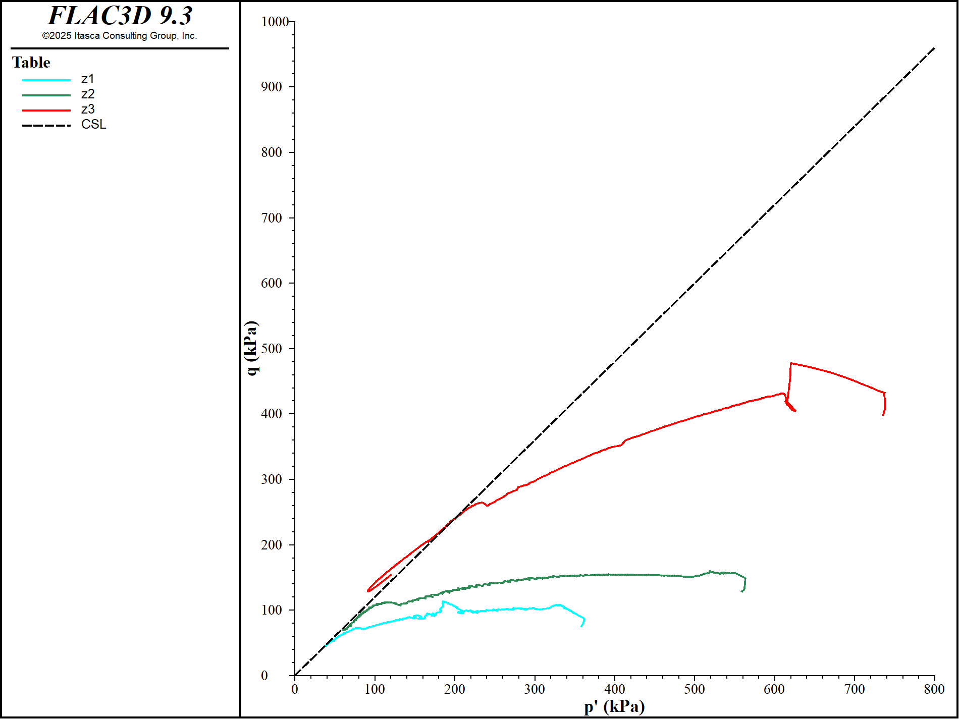
Figure 13: Stress paths of $q$ vs $p'$ of selected zones.

Discussion

For this model with strain-softening material behavior, the results are grid-dependent. This grid-dependence can be checked by increasing or decreasing the global FISH variable “zone_size.” The shear band width shown in Figure 10 will increase or decrease accordingly.

A model’s global behavior is what truly matters when shear banding occurs, because the stress-strain behavior at specific locations can vary, including plastic strain softening, elastic unloading, and even elastic or plastic loading. Only zones within the shear bands may exhibit partial undrained failure paths, which may be mixed with elastic unloading or reloading (see Figure 13). Although the entire model assumes an “undrained” setting, maintaining a strictly undrained condition (constant volume for the soil matrix) is usually not possible for individual zones for two main reasons: (1) the model is not fluid-confined due to the presence of the phreatic surface, and (2) excess pore pressures can be transferred to neighboring zones.

Once the model is in sliding failure, the absolute displacement magnitude is less meaningful because it will continue to increase with further cycling (see Figure 12). However, the accelerating rate of displacement is a good indicator of model instability.

Data File

master.dat

model new
[global zone_size = 1.0]
program call "sketch.dat"
program call "construction.dat"
program call "fluid.dat"
program call "toNorSand.dat"
program call "static.dat"
program call "check.dat"

construction.dat

model restore 'sketch'
;
zone face skin
;
model configure fluid-flow
model large-strain off
model gravity 9.81
;
zone face apply velocity-x 0 range group 'west' ;or 'east' 
zone face apply velocity-y 0 range group 'south' or 'north'
zone face apply velocity (0,0,0) range group 'bottom'
; Null all first
zone null
; Start with just the starter dam
; units in kPa
zone cmodel assign mohr-coulomb range group 'StarterDam'
zone property density 2.0 bulk 3e5 shear 2e5 range group 'StarterDam'
zone property cohesion 20 friction 36 tension 1e20 range group 'StarterDam'
zone initialize-stresses ratio 0.6 range group 'StarterDam'
;
model solve-static convergence 1
model save 'stage-1'
;
; now build up dam layer by layer
[scount_ = 1]
fish define add_layer(mat_,type_)
  scount_ += 1
  if type_ = 'dike' then
    command
      zone cmodel assign mohr-coulomb range group [mat_] 
      zone property density 2.5 bulk 2e5 shear 1.5e5 range group [mat_]
      zone property cohesion 25 friction 32 range group [mat_] 
      zone initialize-stresses ratio 0.6 range group [mat_]
    endcommand
  endif
  if type_ = 'tails' then
    command
      zone cmodel assign mohr-coulomb range group [mat_] 
      zone property density 2.5 bulk 1e5 shear 0.6e5 range group [mat_]
      zone property cohesion 0  friction 28 range group [mat_] 
      zone initialize-stresses ratio 0.8 range group [mat_]
    endcommand
  endif
  command
    model solve-static convergence 1
    ;If saving construction stages
    model save ['stage-' + string(scount_)]
  endcommand
end
; Simulate the construction stages
[add_layer('Tailings01','tails')]
[add_layer('Tailings02','tails')]
[add_layer('Tailings03','tails')]
[add_layer('Dike1','dike')]
[add_layer('Tailings04','tails')]
[add_layer('Dike2','dike')]
[add_layer('Tailings05','tails')]
[add_layer('Dike3','dike')]
[add_layer('Tailings06','tails')]
[add_layer('Dike4','dike')]
[add_layer('Tailings07','tails')]
[add_layer('Dike5','dike')]
[add_layer('Tailings08','tails')]
[add_layer('Dike6','dike')]
[add_layer('Tailings09','tails')]
[add_layer('Dike7','dike')]
[add_layer('Tailings10','tails')]

model save 'construction'

fluid.dat

model restore 'construction'
;
zone gridpoint initialize velocity (0,0,0)
zone gridpoint initialize displacement (0,0,0)
zone initialize state 0
;
zone fluid property porosity 0.3 hydraulic-conductivity 1e-9
zone fluid-density 1
;
zone gridpoint initialize saturation 0
; satuation model is set to cutoff 
zone fluid unsaturated cutoff
;
zone face apply head 57.75 range group 'west'
zone face apply pore-pressure 0 range group 'top'
; 
zone fluid steady-state
model save 'fluid-only'
; now mechanical
model solve-static convergence 1
model save 'fluid'

toNorSand.dat

model restore "fluid"
;
zone gridpoint initialize velocity (0,0,0)
zone gridpoint initialize displacement (0,0,0)
zone initialize state 0
;
zone nodal-mixed-discretization on
; change to NorSand model
zone group 'Tailing' range group 'Tailings01' or 'Tailings02' or ...
    'Tailings03' or 'Tailings04' or 'Tailings05' or 'Tailings06' or ... 
    'Tailings07' or 'Tailings08' or 'Tailings09' or 'Tailings10'
;
zone cmodel assign norsand range group 'Tailing'
zone property shear-reference 2e4 exponent 0.72 range cmodel 'norsand'
zone property pressure-reference 100 poisson 0.15 range cmodel 'norsand'
zone property critical-state-1 .74 critical-state-2 .05 range cmodel 'norsand'
zone property ratio-critical 1.2 range cmodel 'norsand'
zone property factor-coupling 0.25 factor-dilatancy 7.2 range cmodel 'norsand'
zone property hardening-0 45.0 hardening-y 350.0 range cmodel 'norsand' 
zone property flag-inner on range cmodel 'norsand'
zone property state-parameter-initial  0.10 range cmodel 'norsand'
zone property state-parameter-initial -0.10 range group 'Tailings01'
zone property state-parameter-initial -0.10 range group 'Tailings02'
;
fish operator ini_stress(modelName,zp)
  if zone.model(zp) = modelName then
    zone.prop(zp,'stress-xx-initial') = zone.stress.eff(zp)->xx
    zone.prop(zp,'stress-yy-initial') = zone.stress.eff(zp)->yy
    zone.prop(zp,'stress-zz-initial') = zone.stress.eff(zp)->zz
    zone.prop(zp,'stress-xy-initial') = zone.stress.eff(zp)->xy
    zone.prop(zp,'stress-yz-initial') = zone.stress.eff(zp)->yz
    zone.prop(zp,'stress-xz-initial') = zone.stress.eff(zp)->xz
  endif
end
[ini_stress("norsand", ::zone.list)]

model solve-static convergence 1
model save "tonorsand"

static.dat

model restore "tonorsand"
;
zone gridpoint initialize velocity (0,0,0)
zone gridpoint initialize displacement (0,0,0)
zone initialize state 0
; 
zone fluid property pore-pressure-generation on
zone fluid property fluid-modulus 2e5
;
[global iniStep = mech.step]
fish define ramp
  global cycles = mech.step - iniStep
  if cycles < 6000
    ramp = float(cycles)/float(6000)
  else
    ramp = 1.0
  endif
end
; Apply surcharge
zone face apply stress-normal -500 fish ramp range group 'Load'
zone face apply-remove head range group "West"
;
fish define locations
  local v1 = ( -2.5, 0.5, 37.0)
  local v2 = ( 15.5, 0.5, 24.5)
  local v3 = ( 66.3, 0.5, 15.6)
  global z1 = zone.near(v1)
  global z2 = zone.near(v2)
  global z3 = zone.near(v3)
  data.scalar.value(data.scalar.create(v1)) = 1.0
  data.scalar.value(data.scalar.create(v2)) = 1.0
  data.scalar.value(data.scalar.create(v3)) = 1.0
end
[locations]
;
fish define p1
  local sten1 = zone.stress.eff(z1)
  global p1 = tensor.trace(sten1) / (-3.0)
  global q1 = math.sqrt(3.0*tensor.j2(sten1))
  local sten2 = zone.stress.eff(z2)
  global p2 = tensor.trace(sten2) / (-3.0)
  global q2 = math.sqrt(3.0*tensor.j2(sten2))
  local sten3 = zone.stress.eff(z3)
  global p3 = tensor.trace(sten3) / (-3.0)
  global q3 = math.sqrt(3.0*tensor.j2(sten3))
end
history interval 10
fish history name 'cycles' cycles
zone history name='disp-top' displacement position (61,0,60.5)
fish history name 'p1' p1
fish history name 'q1' q1
fish history name 'p2' p2
fish history name 'q2' q2
fish history name 'p3' p3
fish history name 'q3' q3
;
model solve-static cycles 10000
;
history export 'q1' vs 'p1' table 'z1'
history export 'q2' vs 'p2' table 'z2'
history export 'q3' vs 'p3' table 'z3'
table 'CSL' add (0,0) (800,960)
;
model save "static"

Endnote

[1]

This example is listed under the present document title in the i Examples dialog (use the menu command Help -> Examples… to access).