MPAC Examples • Verification
Rough Strip Footing on a Cohesive Frictionless Material (MPAC3D)
Problem Statement
Note
This example is based on the FLAC3D example of the same problem.
The prediction of collapse loads under steady plastic-flow conditions can be difficult for a numerical model to simulate accurately (Sloan and Randolph, 1982). As a two-dimensional example of a steady-flow problem, we consider the determination of the bearing capacity of a strip footing on a cohesive frictionless material (Tresca model). The value of the bearing capacity is obtained when steady plastic flow has developed underneath the footing, providing a measure of the ability of the code to model this condition.
The strip footing is located on an elasto-plastic material with the following properties:
shear modulus (\(G\))
0.1 GPa
bulk modulus (\(K\))
0.2 GPa
cohesion (\(c\))
0.1 MPa
friction angle (\(\phi\))
0°
dilation angle (\(\psi\))
0°
Closed-Form Solution
The bearing capacity obtained as part of the solution to the “Prandtl’s wedge” problem is given by Terzaghi and Peck (1967) as
in which \(q\) is the average footing pressure at failure, and \(c\) is the cohesion of the material. The corresponding failure mechanism is illustrated in the figure below.
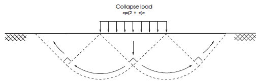
Figure 1: Prandtl mechanism for a strip footing.
MPAC3D Model
For this problem, half-symmetry and plane-strain conditions are assumed in the numerical simulation. The domain used for the analysis is sketched below.
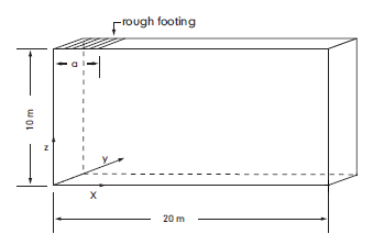
Figure 2: Domain for FLAC3D and MPAC3D half-symmetry simulation.
The area representing the strip footing has a half-width \(a\) of 3 m, the far \(x\)-boundary is at a distance of 20 m from the axis of symmetry, and the far \(z\)-boundary is located 10 m below the footing. The thickness of the domain is selected as 0.25 m to coincide with the zone and background mesh node (i.e., mpoint node) spacing. For a fair comparison, these spacings are kept uniform. In MPAC3D, the footing region is modeled by applying velocity fixity conditions to the mpoint nodes, similar to the velocity fixity applied to FLAC3D zone gridpoints. In this case, all mpoint nodes extending vertically from the footing are fixed and the out-of-balance forces are summed for these nodes to determine the load. This is important as the interpolation footprint may extend to multiple rows of mpoint nodes if using quadratic interpolation.
The mpoint node spacing is set to 0.25, and the mpoint discretization has eight material points per background cell, with a total of 25,600 mpoints.
The boundary conditions applied to the domain are sketched in the next figure. The displacement is restricted in the \(y\)-direction (2D plaine-strain conditions) by fixing the \(y\)-velocity of all mpoint nodes and gridpoints.
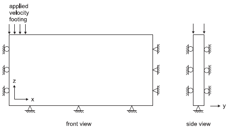
Figure 3: Boundary conditions for MPAC3D analysis—half symmetry.
When using a grid-based numerical method, such as FLAC3D, with a velocity applied to gridpoints to simulate a footing load, the average footing pressure is found by assuming that the footing effective width is represented by a velocity that varies from the value at the last gridpoint to zero at the next gridpoint. In other words, the effective width of the footing is taken to be \(a\), plus half the zone width adjacent to the footing edge (because forces are exerted on the footing by this zone, it is assumed that the forces are divided equally between this zone’s left and right gridpoints). The effective half-width, \(a_e\), is then
where \(x_l\) is the \(x\)-location of the last applied gridpoint velocity, \(x_{l+1}\) is the \(x\)-location of the gridpoint adjacent to \(x_l\), and \(A\) accounts for the variation. If a linear variation is assumed, then \(A\) = 0.5. In the MPAC3D model, the same reasoning is valid since the load is applied similarly.
A velocity of magnitude 0.5 × 10⁻⁵ m/step is applied to the footing for a total of 25,000 calculation steps. Although MPAC3D can model large deformation, the small strain option is used in this example (see model large-strain), enabling direct comparison between MPAC3D, FLAC3D and the analytical bearing capacity.
Results and Discussion
The above MPAC3D model is created alongside a comparable FLAC3D model. A direct comparison of the evolving displacement and stress fields, as well as the load-displacment curve, is possible. The load-displacement curve corresponding to the numerical simulation is presented in Figure 4, in which Normalized Load is the average footing pressure \(p\), normalized by the cohesion \(c\):, \(p/c\), and Displacement is the magnitude of the vertical displacement at the center of the footing. The bearing capacity predicted by FLAC3D is \(q\) = 513.9 kPa, and that predicted by MPAC3D is \(q\) = 492.8 kPa, after 25,000 cycles. When compared to the analytical value of 514.2 kPa, the error is less than 1% for the FLAC3D model and less than 5% for the MPAC3D model. The reason for the larger error in the MPAC model is that quadratic spline interpolation is used, meaning that the area of the footing is effectively different.
The apparent width of the footing is taken to be 3 m, plus half the zone width adjacent to the footing edge (because forces are exerted on the footing by this zone, it is assumed that the forces are divided equally between left and right gridpoints). The error in the bearing capacity is related to the indeterminacy in the apparent width of the footing. The mechanism illustrated in Figure 1 implies a velocity singularity at the ends of the footing. In a numerical simulation, this singularity is spread over the width of one zone. The apparent position of the velocity jump within that zone depends on the exact geometry of the velocity field that develops. In deriving \(q\), it is assumed that the jump occurs half a zone width from the end of the controlled boundary segment (\(A\) = 0.5 in Figure 2); for finer grids, the indeterminacy in footing width decreases, and the match to the exact solution improves.
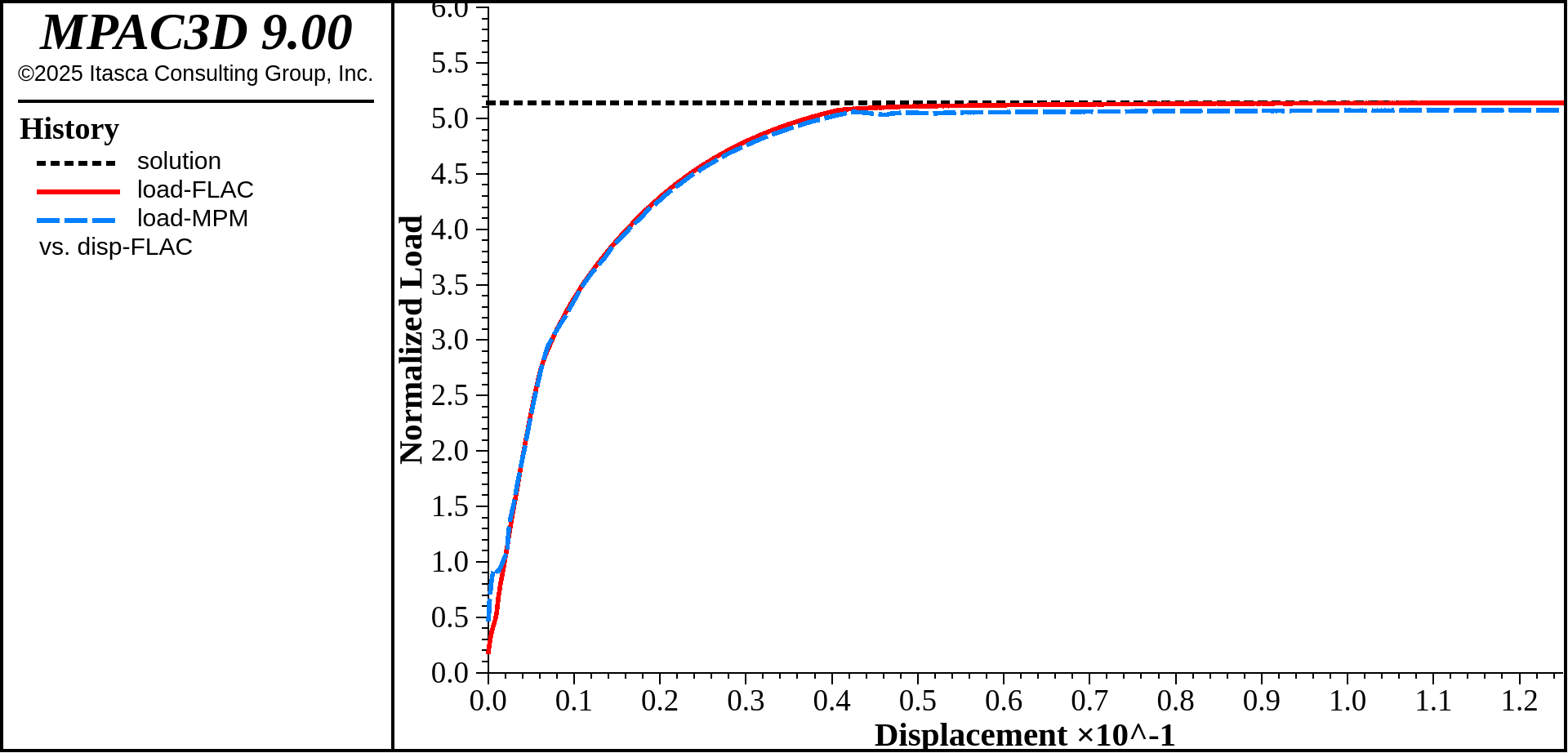
Figure 4: Load-displacement curve showing the results from FLAC3D and MPAC3D against the analytical solution.
The displacement contours at the end of the run are presented in Figure 5, showing good agreement between MPAC3D (right) and FLAC3D (left) and with the mechanism in Figure 1. Note that the plotted FLAC3D displacement field is interpolated from the gridpoints to provide a smooth contour. The MPAC3D results, however, are not interpolated and plotted per mpoint.
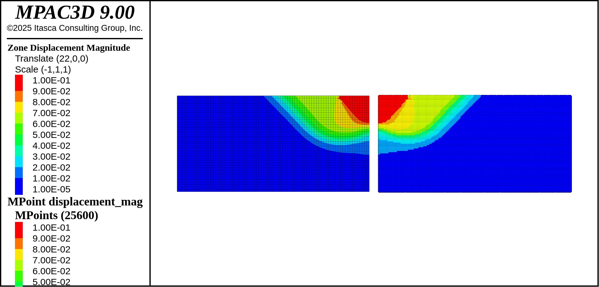
Figure 5: Displacement field at collapse load predicted by MPAC3D (right) and FLAC3D (left).
The vertical stress (\(zz\)-stress) constour is shown in Figure 6 showing good agreement between MPAC3D (right) and FLAC3D (left). Note that neither the FLAC3D or MPAC3D contours are smoothed.
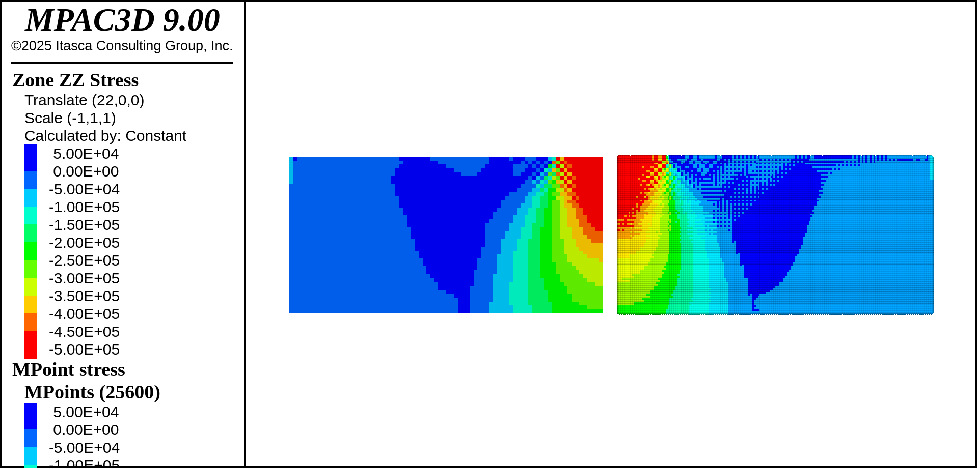
Figure 6: Stress contour (\(zz\)-stress) at collapse load predicted by MPAC3D (right) and FLAC3D (left).
References
Sloan, S. W., and M. F. Randolph. “Numerical Prediction of Collapse Loads Using Finite Element Methods,” Int. J. Num. & Analy. Methods in Geomech., 6, 47-76 (1982).
Terzaghi, K., and R. B. Peck. Soil Mechanics in Engineering Practice, 2nd Ed. New York: John Wiley and Sons (1967).
break
Data File
PrandtlsWedge.dat
;---------------------------------------------------------------------
; 2D rough strip footing on Tresca material (Prandtl's wedge problem)
;---------------------------------------------------------------------
model new
model large-strain off
; Create zones uniformly for fair comparison between mpoints and zones
zone create brick size 80 1 40 point 0 = 0.0,  0.0,  0.0 ...
                               point 1 = 20.0, 0.0,  0.0 ...
                               point 2 = 0.0,  0.25, 0.0 ...
                               point 3 = 0.0,  0.0,  10.0

; Copy zones for mpoints
zone copy -21 0 0

; Assign constitutive model and properties to zones
zone cmodel assign mohr-coulomb
zone property bulk 2.e8 shear 1.e8 cohesion 1.e5 density 1
zone property friction 0. dilation 0. tension 1.e10

; Import mpoints, including all properties and constitutive models.
model domain extent (-24 2) (-2 2) (-3 13)
mpoint node spacing 0.25
mpoint import from-zones range position-x -22 0

; Fix the out-of-plane velocities
zone gridpoint fix velocity-y
mpoint node fix velocity-y

; Loading rate
[global rate = vector(0,0,-0.5e-5)]

; Boundary Conditions - zones
zone face group 'Footing' range position-x 0 3 position-z 10
zone gridpoint fix velocity-x range position-x 0
zone gridpoint fix velocity range union position-x 20 position-z 0
zone gridpoint fix velocity [rate] range group 'Footing'

; Boundary Conditions - mpoint nodes
mpoint node group 'Footing' range position-x -21 -18 position-z 9.9 100 ;position-y 0 0.25
mpoint node fix velocity [rate] range group 'Footing'
mpoint node fix velocity-x range position-x -100 -20.9
mpoint node fix velocity range position-z -100 0.1
mpoint node fix velocity range position-x -1.1 100

; Setup for recording loads
[global gpList = gp.list(gp.isgroup(::gp.list,'Footing'))]
[global mpNList = mpoint.node.group.list('Footing')]
[global cohesion = zone.prop(zone.head,'cohesion')]
[global solution = (2.0 + math.pi)]

; Measure loads
fish define loadFlac
    loadFlac = list.sum(gp.force.unbal(::gpList)->z) / (cohesion) * 1.25
    dispFlac = -gp.disp(gpList(1))->z
    loadMPM = list.sum(mpoint.node.force.unbal(::mpNList)->z) / (cohesion) * 1.25
end
fish history name 'solution' solution
fish history name 'load-FLAC' loadFlac
fish history name 'disp-FLAC' dispFlac
fish history name 'load-MPM' loadMPM
; Linear interpolation for fair comparison
mpoint interpolation linear
; Turn on the volumetric locking adjustment
mpoint locking-adjustment on
; Cycle
model cycle 25000
| Was this helpful? ... | Itasca Software © 2024, Itasca | Updated: Nov 23, 2025 |
