The source code for this example is basic_python.py
Introduction to Python Programming
This section gives a brief introduction to Python programming not specific to using Itasca software. There are many on-line and published resources to find more information:
- The official Python web page: http://python.org.
- The official Python tutorial is a good place to start: https://docs.python.org/3/tutorial/
- http://learnpythonthehardway.org/book/
- Learning Python by Mark Lutx published by O’Reilly.
- For scientific programming specific information see: https://scipy-lectures.github.io/
IPython Console
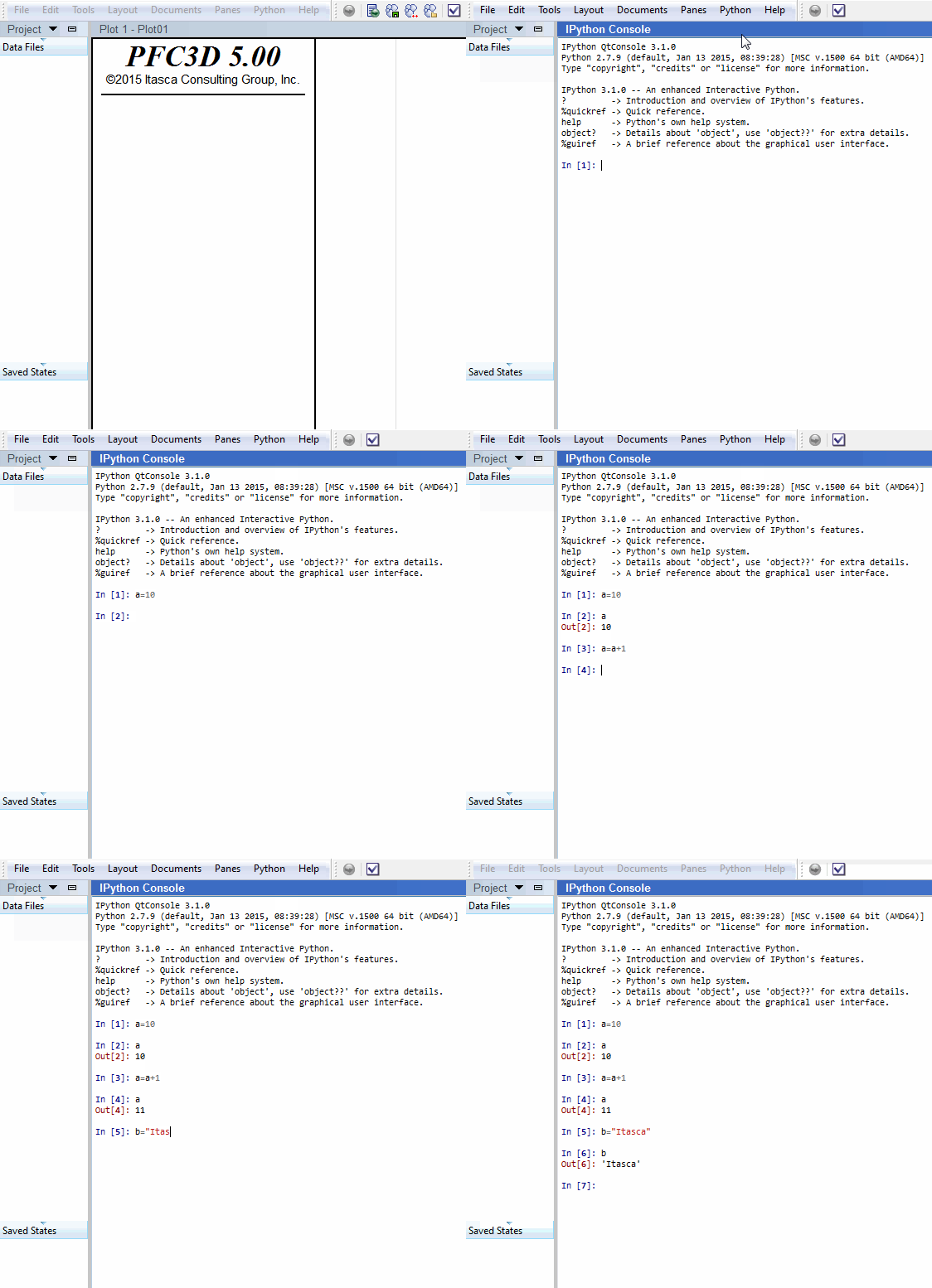
The best way to get started with Python programming is to experiment with the IPython Qt console in PFC. A window like the one shown below is part of the PFC Graphical User Interface. The following examples can be run in this terminal.

- Use the up and down arrow keys to access previous inputs.
- Use the tab key for completion of Python names.
- See http://ipython.org for more information about this terminal.
Basic Types
Every value in Python has a specific type. The most common types are
int, float and str which represent an integer, a real
number and a character string. Below we assign some values to some variables.
size = 0.5
box_count = 10
first_name = "Fred"
last_name = 'Baker'

long_string = """
This is a multi-line string.
Triple quotes are used to define strings like this.
"""
Lists, Tuples and Dictionaries
Three fundamental container types are commonly used in Python. These
are the list, tuple and dict types.
Lists are created with the [ and ] characters.
id_list = [1, 2, 3, 4]
Typing id_list in the IPython console will show us the value of this list
id_list
- output:
[1, 2, 3, 4]
Add an item to the end of a list with the append method.
id_list.append(903)
id_list
- output:
[1, 2, 3, 4, 903]
Iterate over a list (or any sequence) like this,
for id_number in id_list:
    print("id #: ", id_number)
- output:
id #:  1
id #:  2
id #:  3
id #:  4
id #:  903
The
forkeyword is used to loop over a sequences. Note that
white space is used to indicate what code is included in the loop.
Get the length of a list,
len(id_list)
- output:
5
Access individual elements of a list,
id_list[0]
- output:
1
access a sequence of elements (a slice) of a list,
id_list[1:3]
- output:
[2, 3]
The list index can be negative, which returns elements from the back of the list
id_list[-1]
- output:
903
Change the value of the element of a list
id_list[0] = 10.0

print(id_list)
- output:
[10.0, 2, 3, 4, 903]
Lists can store objects of different types,
id_list.append("this is a string")
id_list
- output:
[10.0, 2, 3, 4, 903, 'this is a string']
Tuples
Tuples are like lists but they cannot be changed after being created. In other words tuples are immutable.
parts = (1,2,3,4,5)
parts
- output:
(1, 2, 3, 4, 5)
Dictionaries
Python dictionaries are used for one to one mappings between
objects (key, value pairs). The following line shows a dictionary
literal which we assign to the variable telephone_directory
telephone_directory = {"Jim" : 125, "Steve": 128, "Bob" : 144}
telephone_directory
- output:
{'Jim': 125, 'Steve': 128, 'Bob': 144}
Look up a value in a dictionary,
telephone_directory["Jim"]
- output:
125
Add values to an existing dictionary,
telephone_directory["Fred"] = 147
telephone_directory[(1,3)] = 0.22344
telephone_directory
- output:
{'Jim': 125, 'Steve': 128, 'Bob': 144, 'Fred': 147, (1, 3): 0.22344}
Remove key, value pairs from a dictionary
del(telephone_directory["Bob"])
Iterate over a the key, value pairs of a dictionary
for key, value in telephone_directory.items():
    print("found key: {} with value: {}".format(key, value))
- output:
found key: Jim with value: 125
found key: Steve with value: 128
found key: Fred with value: 147
found key: (1, 3) with value: 0.22344
Or get a list of the keys.
telephone_directory.keys()
- output:
dict_keys(['Jim', 'Steve', 'Fred', (1, 3)])
For more about dictionaries see: The dictionary section of the Python tutorial
Defining Functions
Functions are defined in Python with the def keyword,
def my_function(a, b):
    return a + b
my_function(1.0, 5)
- output:
6.0
Error Handling in Python.
Here we are going to deliberately make a mistake so we can show how Python handles errors.
my_function(1.0, "This is a Python string")
- output:
Traceback (most recent call last):
  File "<string>", line 8, in <module>
  File "", line 1, in <module>
  File "c:/src/ppfc/common/python/src/basic_python.py", line 60, in <module>
    my_function(1.0, "This is a Python string")
  File "c:/src/ppfc/common/python/src/basic_python.py", line 49, in my_function
    return a + b
TypeError: unsupported operand type(s) for +: 'float' and 'str'
There is no way to add float and str objects in python so we
get an error message. Causing an error in Python results in a
traceback being printed. The traceback tells you the type of error
encountered and the line and file the error occured in.
Note
For advanced troubleshooting use the Python debugger. Typing debug in
the IPython console activates the debugger.
Object-Oriented Programming
In Python all values (values are things variables can refer too) are
objects. Objects are instances of a class. Objects have methods. For
example our long_string variable is an object of type str.
Next we call a method of the str objects referred to by the
variable long_string,
long_string = """
This is a multi-line string.
Triple quotes are used to define strings like this.
"""
long_string.split()
- output:
['This', 'is', 'a', 'multi-line', 'string.', 'Triple', 'quotes', 'are', 'used', 'to', 'define', 'strings', 'like', 'this.']
In this case we are calling the split method of the str object and
it returns a list of strings split along the spaces. In the PFC Python
bindings, model objects are represented as objects. For example there
is a Ball object to represent PFC Balls. This is described more fully
in the next section.
Interactive Documentation
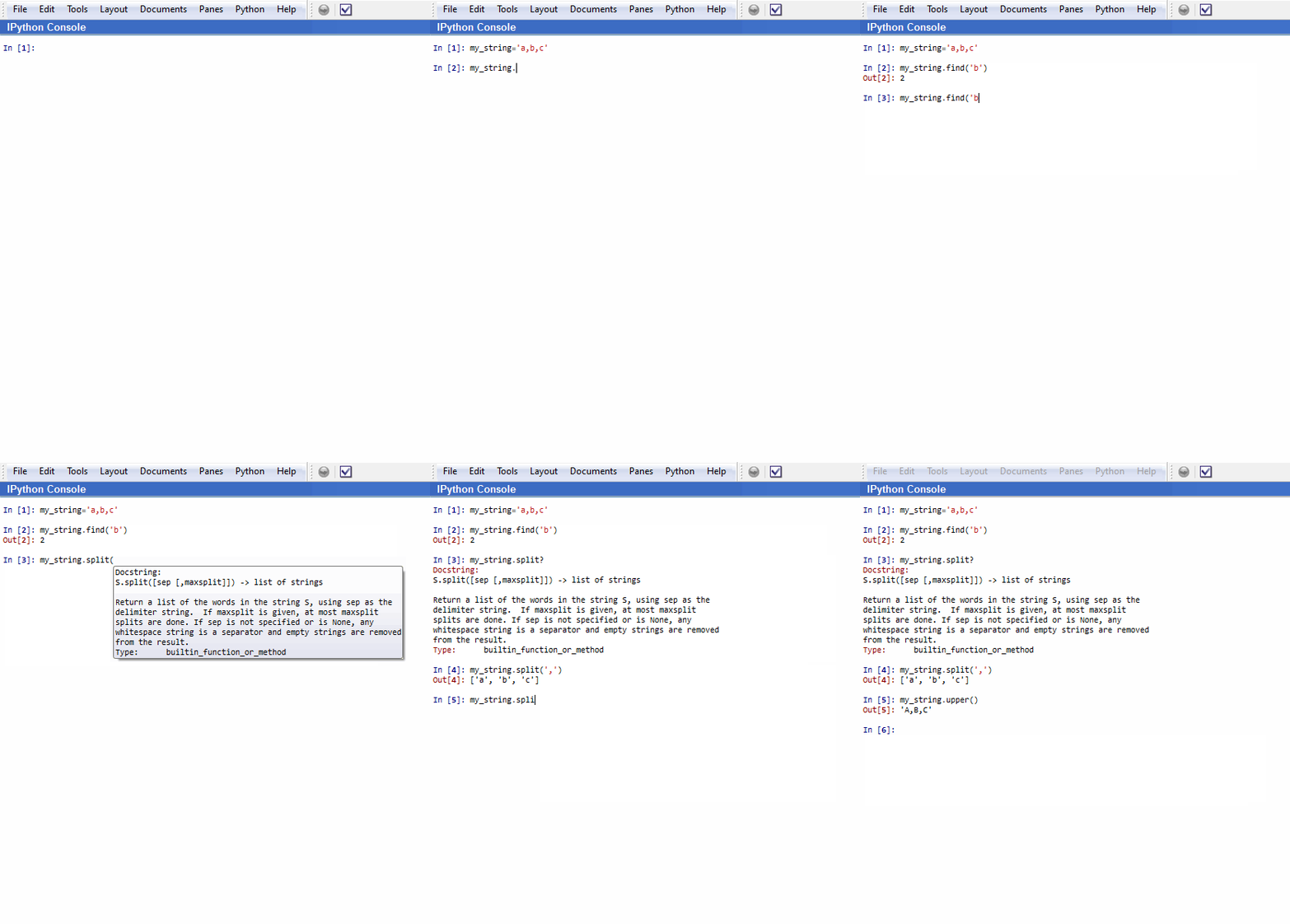
The IPython console displays interactive completion and inline documentation to make programming easier. The following figure uses these features to show some of the available methods of string objects.
- Pressing the
tabkey at the end of a partially written name will offer interactive completions. Pressingtabagain will cycle through the available names. Pressingenterselects a completion. - Interactive documentation is shown when the
(character is typed after a function name. - Alternatively, adding a
?character to the end of any Python function, module or object displays inline documentation.

Array Style Programming with NumPy
This section describes a NumPy array-based interface to work with PFC and FLAC3D models from Python. Instead of dealing with individual Ball, Zone, or Gridpoint objects, the array interface deals with the attributes and properties of all balls, zones, or gridpoints simultaneously. This is often considerably faster than looping over the list of individual objects.
Note
NumPy is an extension to Python which defines a powerful array object and many useful numerical operations. Using NumPy and array style programming can be much faster than looping natively in Python. The style of programming is different from that defined in the object-oriented interface.
For more information about NumPy see: http://numpy.org
NumPy Basics
import numpy as np
The numpy module is a third-party extension to Python, but it is
included in the FLAC3D Python environment. It is conventional to
import this module by the shortened name np.
Most of this tutorial demonstrates using Python functions provided by
Itasca which return numpy arrays or accept numpy arrays as
arguments. A short overview of the basics of the numpy module is
given first.
Arrays can be created several ways.
np.array([1,2,3,4,5])
- output:
[1 2 3 4 5]
np.linspace(0,1,15)
- output:
[ 0.          0.07142857  0.14285714  0.21428571  0.28571429  0.35714286
  0.42857143  0.5         0.57142857  0.64285714  0.71428571  0.78571429
  0.85714286  0.92857143  1.        ]
np.zeros((4,4))
- output:
[[ 0.  0.  0.  0.]
 [ 0.  0.  0.  0.]
 [ 0.  0.  0.  0.]
 [ 0.  0.  0.  0.]]
a = np.linspace(0,1,15)
b = np.ones_like(a)
a + b
- output:
[ 1.          1.07142857  1.14285714  1.21428571  1.28571429  1.35714286
  1.42857143  1.5         1.57142857  1.64285714  1.71428571  1.78571429
  1.85714286  1.92857143  2.        ]
a + 1e-2 * b
- output:
[ 0.01        0.08142857  0.15285714  0.22428571  0.29571429  0.36714286
  0.43857143  0.51        0.58142857  0.65285714  0.72428571  0.79571429
  0.86714286  0.93857143  1.01      ]
np.sin(a)
- output:
[ 0.          0.07136785  0.14237173  0.21264953  0.28184285  0.34959881
  0.41557185  0.47942554  0.54083421  0.5994847   0.6550779   0.70733028
  0.75597537  0.80076507  0.84147098]
In the second example above, notice that the value 1e-2 is broadcast
to the dimension of the array b.
Arithmetic on arrays is much faster that looping over the individual components of an array and performing some operation. Nearly all types of looping or iteration over arrays can be expressed by array operations.
print(a[0])
a[0] = 20.2
print(a)
- output:
0.0
[ 20.2          0.07142857   0.14285714   0.21428571   0.28571429
   0.35714286   0.42857143   0.5          0.57142857   0.64285714
   0.71428571   0.78571429   0.85714286   0.92857143   1.        ]
Multidimensional array are commonly used in the Itasca array interfaces.
c = np.array(((1,2,3),(4,5,6),(7,8,9),(10,11,12)))
print(c)
- output:
[[ 1  2  3]
 [ 4  5  6]
 [ 7  8  9]
 [10 11 12]]
The individual components of a multidimensional array can be accessed several ways
c[0][0]
- output:
1
c[:,0]
- output:
[ 1 4 7 10]
xcomp, ycomp, zcomp = c.T
print(xcomp)
- output:
[ 1 4 7 10]
A common point of confusion with numpy is the concept of array
views. In this case the variable xcomp is a view into the array
c. Changing xcomp will change c.
xcomp[0] = 12345.5
print(c)
c[0][0] = 1.0
- output:
[[12345     2     3]
 [    4     5     6]
 [    7     8     9]
 [   10    11    12]]
To avoid this, make copy of the view.
d = np.copy(c[:,0])
print(c)
- output:
[[ 1  2  3]
 [ 4  5  6]
 [ 7  8  9]
 [10 11 12]]
Now changing d will not change c.
d[0] = 99.99
print(c)
- output:
[[ 1  2  3]
 [ 4  5  6]
 [ 7  8  9]
 [10 11 12]]
The numpy module defines many powerful functions for working with
arrays of multidimensional data.
| Was this helpful? ... | PFC 6.0 © 2019, Itasca | Updated: Nov 19, 2021 |
