FLAC3D Theory and Background • Constitutive Models

Plastic-Hardening Model

The Plastic-Hardening (PH) model is a shear and volumetric hardening constitutive model for the simulation of soil behavior. When subjected to deviatoric loading (e.g., during a conventional drained triaxial test), soils usually exhibit a decrease in stiffness, accompanied by irreversible deformation. In most cases, the plot of deviatoric stress versus axial strain obtained in a drained triaxial test may be approximated by a hyperbola. This feature was discussed by Duncan and Chang (1970) in their well-known “hyperbolic-soil” model, which is formulated as a non-linear elastic model. The PH model is formulated within the framework of hardening plasticity (Schanz et al. 1999) allowing the removal of the main drawbacks of the original non-linear elastic model formulation (e.g., detection of loading/unloading pattern, non-physical bulk modulus).

The main features of the PH model are:

1. hyperbolic stress-strain relationship during axial drained compression;
2. plastic strain in mobilizing friction (shear hardening);
3. plastic strain in primary compression (volumetric hardening);
4. stress-dependent elastic stiffness according to a power law;
5. elastic unloading/reloading compared to virgin loading;
6. memory of pre-consolidation stress; and
7. Mohr-Coulomb failure criterion.

The model is straightforward to calibrate using either conventional lab tests or in-situ tests. It is well established for soil-structure interaction problems, excavations, tunneling, and settlements analysis, among many other applications.

In this section, principal stress, \(\sigma_i\), and strain, \(\varepsilon_i\), i = 1,3, components are positive in tension. Also, all stresses are effective by default if not explicitly stated. The principal effective stresses are with the order \(\sigma_1 \le \sigma_2 \le \sigma_3\), and \(\sigma_1\) is the most compressive stress.

Incremental Elastic Law

The PH model adopts hypo-elasticity for the description of elastic behavior,

(1)\[ \Delta p = -K \Delta \epsilon^e_v\]

(2)\[ \Delta s_{ij} = 2G \Delta \epsilon_{ij}\]

where \(p\) is the mean pressure defined as \(p = − \sigma_{ii}/3\), \(\epsilon^e_v\) is the volumetric elastic strain defined as \(\epsilon^e_v = \varepsilon^e_{ii}\), \(s_{ij} = \sigma_{ij} + p \delta_{ij}\) and \(\epsilon_{ij} = \varepsilon_{ij} - (\epsilon_v/3)\delta_{ij}\) are the deviatoric stress tensor and deviatoric elastic strain tensor, respectively. \(\delta_{ij}\) is defined as \(\delta_{ij} = 1\) if \(i = j\) and \(\delta_{ij} = 0\) if \(i \ne j\). \(K\) and \(G\) are the elastic bulk and shear moduli, which can be derived from the elastic unloading-reloading Young’s modulus, \(E_{ur}\), and the unloading-reloading Poisson’s ratio, \(\nu\), are obtained using the relations:

(3)\[ K = {E_{ur} \over {3(1-2\nu)}}\]

(4)\[ G = {E_{ur} \over {2(1+\nu)}}\]

In the PH model, the Poisson’s ratio is assumed to be a constant with a typical value of 0.2 (if otherwise not provided at input).

The Young’s modulus is a stress-dependent parameter:

(5)\[E_{ur} = E^{ref}_{ur} Z^m\]

where

(6)\[Z = {{c \cot \phi - \sigma_3} \over {c \cot \phi + p^{ref}}} \ge f_{cut}\]

and \(E^{ref}_{ur}\), \(m\), \(c\), \(p^{ref}\), and \(\phi\) are user-defined constant parameters. \(E^{ref}_{ur}\) is the reference unloading-reloading stiffness modulus at the reference pressure \(p^{ref}\). The current unloading-reloading stiffness modulus \(E_{ur}\) depends on the maximum (minimum compressive) principal stress, \(\sigma_3\), the cohesion, \(c\), and the ultimate friction angle, \(\phi\), as well as the power, \(m\). For clays, \(m\) is usually close to 1. For sands, \(m\) is usually between 0.4 and 0.9. The default cut-off factor \(f_{cut}\) is 0.1.

The PH model also employs an additional stiffness measure, \(E_{50}\), which defines the initial slope of the hyperbolic stress-strain curve (see Equation (7) and Figure 1). Parameter \(E_{50}\) obeys the following power law:

(7)\[E_{50} = E^{ref}_{50} Z^m\]

Here \(E^{ref}_{50}\) is a material parameter, which could be estimated from a set of triaxial compression tests with various cell stresses.

Shear Yield Criterion and Flow Rule

The shear yield function determining the onset and development of shear hardening is defined as

(8)\[f^s = {{E_{ur}} \over {E_i}} \cdot {{q_a q} \over { (q_a - q)}} - q - {{E_{ur} \gamma^p} \over 2} = 0\]

where \(\gamma^p\) is a shear hardening parameter (one of the internal variables) defined in (13), \(E_i = 2 E_{50} / (2 − R_f)\), \(q = \sigma_3 − \sigma_1\), and \(q_a\) is given as

(9)\[q_a = {{q_f} \over {R_f}} = K_{qa} (c \cot \phi - \sigma_3)\]

where

(10)\[K_{qa} = {{1} \over {R_f}} \cdot {{2 \sin \phi} \over {1 - \sin \phi}}\]

The failure ratio \(R_f = q_f / q_a\) has a value smaller than 1 (typically, \(R_f\) = 0.9 is used). Note that the ultimate deviatoric stress, \(q_f\), is defined as

(11)\[q_f = {{2 \sin \phi (c \cot \phi - \sigma_3)} \over {1 - \sin \phi}}\]

is consistent with the Mohr-Coulomb failure criterion (Figure 1).

For a standard drained triaxial test, the connection between the axial (vertical compressional) strain, \(\varepsilon_1\), and deviatoric stress, \(q\), can be described by a hyperbolic relation:

(12)\[\varepsilon_1 = {{q_a q} \over {E_i (q_a - q)}}\]

Equation (12) is graphically represented in Figure 1 with the cut-off at \(q_f\).

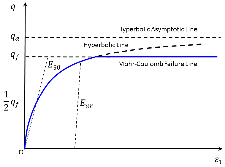
Figure 1: Hyperbolic stress-strain relation in primary shear loading.

The shear hardening parameter \(\gamma^p\) is defined so that its incremental form is:

(13)\[\Delta \gamma^p = - (\Delta \varepsilon^p_1 - \Delta \varepsilon^p_2 - \Delta \varepsilon^p_3)\]

Due to the increase of \(\gamma^p\), the shear yield surface will expand up to the ultimate surface, which is defined by the conventional Mohr-Coulomb failure criterion. In case the material experiences ultimate shear failure, the conventional Mohr-Coulomb failure criterion applies.

The PH model uses the following flow rule between volumetric and shear plastic strains:

(14)\[\Delta \varepsilon^p_v = \sin \psi_m \Delta \gamma^p\]

where \(\sin \psi_m\) is the mobilized dilation angle, which should be smaller or equal to the user-defined ultimate dilation angle \(\psi\). The mobilized dilation angle is based on Rowe’s dilation law (1962):

(15)\[\sin \psi_m = F_c {{\sin \phi_m - \sin \phi_{cv}} \over {1 - \sin \phi_m \sin \phi_{cv}}} \mbox{\;,\;\;if\;} \sin \phi_m < \sin \phi_{cv}\]

(16)\[\sin \psi_m = {{\sin \phi_m - \sin \phi_{cv}} \over {1 - \sin \phi_m \sin \phi_{cv}}} \mbox{\;,\;\;if\;} \sin \phi_m \ge \sin \phi_{cv}\]

where the parameter \(F_c\) is a contraction scale factor, with the allowable range of 0 to 0.25 and default value of 0.0 for most soils if the contraction is not considered. The critical state friction angle \(\phi_{cv}\) is defined as

(17)\[\sin \psi_{cv} = {{\sin \phi - \sin \psi} \over {1 - \sin \phi \sin \psi}}\]

The mobilized friction \(\phi_m\) is defined in terms of the current stress state

(18)\[\sin \phi_m = {{\sigma_1 - \sigma_3} \over {\sigma_1 + \sigma_3 - 2c \cot \phi}}\]

A non-associated flow rule consistent with the Mohr-Coulomb yield criterion is used in the model. The shear potential function is defined as

(19)\[g^s = m_1 \sigma_1 + m_3 \sigma_3\]

where \(m_1 = (-1+\sin \psi_m)/2\) and \(m_3 = (1+\sin \psi_m)/2\).

In order to avoid over-dilatancy when the soil reaches its critical void state at \(e_{max}\), the dilation angle needs a minor modification. One way proposed by Schanz et al. (1999) is to set a cut-off rule, so that

(20)\[\sin \psi_m^{cut} = 0 \mbox{, if } e \ge e_{max}\]

Here we introduce a smoothing technique to avoid a sudden change of dilation angle:

(21)\[\sin \psi_m^{smooth} = 100 \left( 1 - {e \over {e_{max}}} \right) \sin \psi_m \mbox{, if } e \ge 0.99 e_{max}\]

The dilation rules with cut-off, smoothing technique, and without dilation cut-off are schematically compared in Figure 2.

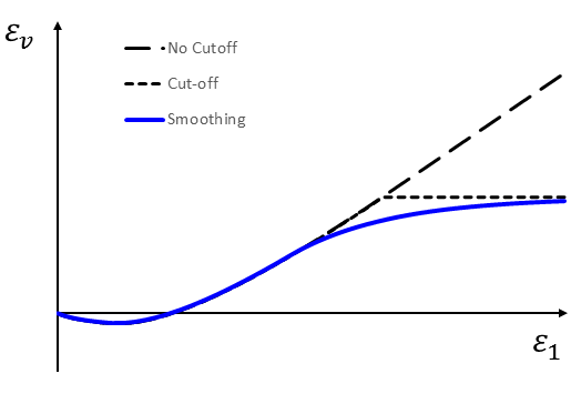
Figure 2: Volumetric strain curve for a standard triaxial compression test with dilation cut-off and smoothing.

Volumetric Cap Criterion and Flow Rule

The volumetric (cap) yield function is defined as

(22)\[f^v = g^v = {{\tilde{q}^2} \over {\alpha^2}} + p^2 -p^2_c = 0\]

where \(\alpha\) is a constant derived internally from other material parameters based on a virtual (numerical) oedometer test, \(\tilde{q}\) is a shear stress measure defined as \(\tilde{q} = − [\sigma_1 + (\delta - 1)\sigma_2 − \delta \sigma_3]\), and \(\delta = (1 + \sin \phi)/(1 − \sin \phi)\). The initial value of hardening parameter \(p_c\), which denotes the preconsolidation pressure, can be determined using the initial stress state and over-consolidation ratio, \(OCR\), so that

(23)\[p_{c,ini} = OCR \cdot \sqrt{{{\tilde{q}^2_{ini}} \over {\alpha^2}} + p^2_{ini}}\]

If \(OCR\) has a large value, the model behaves as if there is no cap present. The associated flow rule is adopted for volumetric hardening, which means that the potential volumetric function is assumed to be the same as the volumetric yield function (see Equation (24)).

The volumetric hardening parameter \(\gamma^v\) (one of the internal variables) is defined incrementally as

(24)\[\Delta \gamma^v = - \Delta \varepsilon^p_v = - (\Delta \varepsilon^p_1 + \Delta \varepsilon^p_2 + \Delta \varepsilon^p_3)\]

where \(\Delta \varepsilon^p_v\) is the volumetric plastic strain increment.

Evolution of the hardening parameter, \(p_c\), is given by the relation:

(25)\[\Delta p_c = H_c \left( {c \cot \phi + p_c} \over {c \cot \phi + p^{ref}} \right)^m \Delta \gamma^v\]

where \(H_c\) is a constant parameter that can be derived internally from other material parameters. Instead of taking \(\alpha\) and \(H_c\) as input material parameters, another two parameters, \(K_{nc}\) and \(E^{ref}_{oed}\) are specified as input. Parameter \(K_{nc}\) denotes normal consolidation coefficient and \(E^{ref}_{oed}\) stands for the tangent oedometer stiffness at the reference pressure \(p^{ref}\). If \(K_{nc}\) is not provided by the user, it is taken as \(K_{nc} = 1 − \sin \phi\) (default value). The PH model reserves the flexibility for the user to input user-defined \(\alpha\) and \(H_c\) instead of internal calculation for \(\alpha\) and \(H_c\). A typical value for \(\alpha\) is between 0.6 and 2.0 for most soils. Parameter \(H_c\) is calculated as \(H_c = k K_p\), where \(k\) is a correction factor with a typical value of \(0 < k \le 1\), \(K_p = K_1 K_2 / (K_1 - K_2)\), \(K_1 = E^{ref}_{ur} / [3(1-2\nu)]\), and \(K_2 = E^{ref}_{oed} (1 + 2 K_{nc})/3\). Specifically, \(k\) = 1 if at isotropic compression state.

Tensile Yield Criterion and Flow Rule

The model checks for the tension failure condition. The tension failure and potential functions are

(26)\[f^t = g^t = \sigma_3 - \sigma^t\]

where \(\sigma^t\) is the tension limit. By default, \(\sigma^t\) is zero and the user can provide a value with an upper limit of \(c/\tan \phi\). The model does not consider tension hardening.

Plastic Corrections

In the implementation of the PH model, elastic trial stresses, \(\sigma^I_{ij}\), are first computed by adding to the old stresses, \(\sigma^o_{ij}\), elastic increments computed using the total strain increment \(\Delta \varepsilon_{ij}\) for the step (see Eq. (1.395)). During this step, the moduli and mobilized dilation angle are assumed to be constants (for simplicity) and calculated based on the old stress components. All stresses are assumed to be effective.

The formulation for the trial stresses (denoted by a superscript \(I\)) in principal axes are:

(27)\[\begin{split}\begin{matrix} \sigma^I_1 = \sigma^o_1 + \alpha_1 \Delta \varepsilon_1 + \alpha_2 \Delta \varepsilon_2 + \alpha_3 \Delta \varepsilon_3 \\ \\ \sigma^I_2 = \sigma^o_2 + \alpha_1 \Delta \varepsilon_2 + \alpha_2 \Delta \varepsilon_3 + \alpha_3 \Delta \varepsilon_1 \\ \\ \sigma^I_3 = \sigma^o_3 + \alpha_1 \Delta \varepsilon_3 + \alpha_2 \Delta \varepsilon_1 + \alpha_3 \Delta \varepsilon_2 \end{matrix}\end{split}\]

where \(\alpha_1 = K +4G/3\), \(\alpha_2 = K −2G/3\), \(K\) and \(G\) are the tangent elastic bulk and shear modulus, respectively, and (\(\Delta \varepsilon_1, \Delta \varepsilon_2, \Delta \varepsilon_3\)) is the set of principal strain increments.

The trial internal variables, \(\gamma^p\) and \(\gamma^v\) , take their values from the previous step. If the hardening yield criteria (Equation (8) and/or (22)) are exceeded, both the stress components and internal variables will be corrected as described below.

First, consider the situation when only shear hardening occurs, \(f^s > 0\). The plastic strain increment is oriented in the direction of the gradient of the potential function in the principal stress space. Using Equation (19), we get

(28)\[\begin{split}\begin{matrix} \Delta \varepsilon^{ps}_1 = \lambda^s {{\partial g^s} \over {\partial \sigma_1}} = m_1 \lambda^s \\ \\ \Delta \varepsilon^{ps}_2 = \lambda^s {{\partial g^s} \over {\partial \sigma_2}} = 0 \\ \\ \Delta \varepsilon^{ps}_3 = \lambda^s {{\partial g^s} \over {\partial \sigma_3}} = m_3 \lambda^s \end{matrix}\end{split}\]

The shear hardening parameter increment is obtained from Equation (13),

(29)\[\Delta \gamma^p = - \lambda^s (m_1 - m_3) = \lambda^s\]

Thus, the corrected (new) stress components become:

(30)\[\begin{split}\begin{matrix} \sigma_1 = \sigma^I_1 - \lambda^s (\alpha_1 m_1 + \alpha_2 m_3) \\ \\ \sigma_2 = \sigma^I_2 - \lambda^s (\alpha_2 m_1 + \alpha_2 m_3) \\ \\ \sigma_3 = \sigma^I_3 - \lambda^s (\alpha_1 m_3 + \alpha_2 m_1) \end{matrix}\end{split}\]

and the corrected internal variable is

(31)\[\gamma^p = \gamma^{p,I} + \Delta \gamma^p = \gamma^{p,I} + \lambda^s\]

Using Equation (30) and definitions \(m_1\) and \(m_2\) from Equation (19), updated shear stress and parameter \(q_a\) (see Equation (9)) are calculated as

(32)\[q = q^I - 2G \lambda^s\]

(33)\[q_a = q^I_a + K_{qa} (\alpha_1 m_3 + \alpha_2 m_1) \lambda^s\]

After substituting the corrected parameters \(q\), \(q_a\), \(\gamma^p\) into Equation (8), parameter \(\lambda^s\) can be obtained by solving a nonlinear equation \(f^s(\lambda^s)\) = 0 using an iteration method. Note that \(\gamma^p\) in Equation (31) uses the current value of \(\lambda^s\) updated in each iteration step, which implies that the correction algorithm is semi-implicit.

If the trial shear stress exceeds the Mohr-Coulomb shear failure surface, the corrections used in Mohr-Coulomb model implementation apply.

Now consider the case when the elastic guess (Equation (22)) exceeds the volumetric yield criterion, \(f^v > 0\), and the volumetric hardening occurs. The plastic strain increments are related to the gradient of the potential function in the stress space as

(34)\[\begin{split}\begin{matrix} \Delta \varepsilon^{pv}_1 = \lambda^v {{\partial g^v} \over {\partial \sigma_1}} = \left[ - {{2 \tilde{q}} \over {\alpha^2}} - {2 \over 3} p \right] \lambda^v \\ \\ \Delta \varepsilon^{pv}_2 = \lambda^v {{\partial g^v} \over {\partial \sigma_2}} = \left[ - {{2 \tilde{q}} \over {\alpha^2}} (\delta -1) - {2 \over 3} p \right] \lambda^v \\ \\ \Delta \varepsilon^{pv}_3 = \lambda^v {{\partial g^v} \over {\partial \sigma_3}} = \left[ {{2 \tilde{q}} \over {\alpha^2}} \delta - {2 \over 3} p \right] \lambda^v \end{matrix}\end{split}\]

Evolution of the hardening parameter \(\gamma^v\) is given by the relation:

(35)\[\Delta \gamma^v = - \Delta \varepsilon^p_v = 2 p \lambda^v\]

In the above formulation, the plastic strain and volumetric hardening parameter increment are related to the current stress measurement (\(p\) or \(\tilde{q}\)), so the correction algorithm again uses a semi-implicit approach.

The corrected stress components are obtained by analogy with shear hardening,

(36)\[\begin{split}\begin{matrix} \sigma_1 = \sigma^I_1 - \lambda^v \left[ 2pK + {{4 \tilde{q} G} \over {\alpha^2}} \right] \\ \\ \sigma_2 = \sigma^I_2 - \lambda^v \left[ 2pK + {{4 (\delta -1) \tilde{q} G} \over {\alpha^2}} \right] \\ \\ \sigma_3 = \sigma^I_3 - \lambda^v \left[ 2pK - {{4 \delta \tilde{q} G} \over {\alpha^2}} \right] \end{matrix}\end{split}\]

Noting that \(p^{(I)} = −(\sigma_1 + \sigma_2 + \sigma_3)/3\) and \(\tilde{q}^{(I)} = − [\sigma_1 + (\delta - 1)\sigma_2 − \delta \sigma_3]\), and using Equation (36) we get

(37)\[p = {{p^I} \over {1 + 2 K \lambda^v}}\]

(38)\[\tilde{q} = {{\tilde{q}^I} \over {1 + 2 M \lambda^v}}\]

where \(M = 4G(\delta^2 − \delta + 1) / \alpha^2\). After substituting the corrected \(p\) and \(\tilde{q}\) into the yield function \(f^v\), (Equation (22)), parameter \(\lambda^v\) can be obtained by solving the nonlinear equation \(f^v(\lambda^v)\) = 0 for the smallest root using an iterative method.

Finally,we consider the situation when the elastic trial stresses exceed both the shear yield hardening surface and volumetric yield hardening surface. In this case, the plastic strain increment is related to the partial derivatives of the potential functions as follows:

(39)\[\begin{split}\begin{matrix} \Delta \varepsilon^{p}_1 = \lambda^s {{\partial g^s} \over {\partial \sigma_1}} + \lambda^v {{\partial g^v} \over {\partial \sigma_1}} = m_1 \lambda^s + \left[ - {{2 \tilde{q}} \over {\alpha^2}} - {2 \over 3} p \right] \lambda^v \\ \\ \Delta \varepsilon^{p}_2 = \lambda^s {{\partial g^s} \over {\partial \sigma_2}} + \lambda^v {{\partial g^v} \over {\partial \sigma_2}} = \left[ - {{2 \tilde{q}} \over {\alpha^2}} (\delta -1) - {2 \over 3} p \right] \lambda^v \\ \\ \Delta \varepsilon^{p}_3 = \lambda^s {{\partial g^s} \over {\partial \sigma_3}} + \lambda^v {{\partial g^v} \over {\partial \sigma_3}} = m_3 \lambda^s + \left[ {{2 \tilde{q}} \over {\alpha^2}} \delta - {2 \over 3} p \right] \lambda^v \end{matrix}\end{split}\]

Parameters \(\gamma^s\) can \(\gamma^v\) can be found by using an iterative method similar to that adopted in the shear or volumetric hardening correction technique. If the trial stress is out of both the volumetric hardening surface and Mohr-Coulomb failure surface, the Mohr-Coulomb failure function should be used instead of the shear hardening function.

Implementation Procedure

In the initialization step, the initial stress, evolution parameters \(\gamma^s\) can \(\gamma^v\) and strain increment are defined for the zone and are assumed to be constant during this step. For simplicity, the stiffness moduli and dilation, which are dependent on the current stress and evolution parameters, are also assumed to be constant in the zone during this step. The trial elastic stresses and the possible stress corrections are defined at the sub-zone level. The trial stress increments obey the linear elastic (Hooke’s) law. If the trial stresses violate the tension limit, the tension failure procedure is called. The next step is to check whether the tension-corrected stress is in the tension or compression side. If the corrected stress is tensile, volumetric hardening will not apply. In either side, if the stress is out of the shear failure or shear yield surface, the shear failure or hardening procedure will be called, respectively. In the compression side, if the stress is out of the volumetric yield surface, the volumetric hardening procedure will be called. In particular, if the stress is also out of the shear failure or shear yield surface, the mixed procedure with both the volumetric hardening and shear failure/hardening corrections will be called. To ensure the averaged stress in the zone level is within the tension limit, a second tension failure procedure is called if any volumetric hardening or shear hardening/failure occurs. After all sub-zones complete the stress check for tension and shear failure, shear and volumetric hardening criteria, the internal variables, stiffness moduli and dilation are updated based on the zone-averaged stresses.

Comparison of the PH model and CYSoil model

The PH and CYSoil models share many similar features. For example, both models have stress-dependent moduli, both have primary shear and volumetric hardening, both employ a hyperbolic relation for the deviatoric stress versus axial strain during triaxial compression, the volumetric yield and potential functions are the same in both models, etc. However, there are some differences between the models as outlined below.

• For primary shear, the CYSoil model uses a Mohr-Coulomb type yield function associated with the mobilized friction angle, while the PH model uses the yield function described by Equation (19).
• The CYmodel uses the accumulated plastic shear strain as one of the evolution parameters (\(\gamma^p\)), while the definition for \(\gamma^p\) differs from plastic shear strain in the PH model (see Equation (13)).
• The CYSoil model moduli are dependent on the mean pressure, while the PH model moduli are dependent on the maximum principal stress (minimum compressive).
• The PH model introduces a modulus \(E_{50}\) to determine the initial slope of the hyperbolic curve during the triaxial compression, while the CYSoil model does not have such modulus; this implies that these two models may have different hyperbolic curves during the drained triaxial compression, although the ultimate shear stresses are the same.
• In the CYSoil model, the parameter \(\alpha\) is user-defined, while in the PH model, this parameter can be internally calculated using other input parameters.
• A constant ratio between the elastic and plastic volumetric strain is assumed during isotropic compression at any pressure in the CYSoil model, while the PH model does not adopt this assumption. As a result, the hardening law provided by Equation (25) is used in the PH model.
• Most parameters of the PH model can be calibrated through the conventional triaxial and oedometer compression tests (see the next section on calibration), while calibration of the CYSoil model parameters is more elaborate.
• In the CYSoil model, many parameters can be input through tables. Currently, the PH model does not have this flexibility feature.

Calibration of Material Parameters Using Laboratory Data

This section presents information on calibration techniques for the PH model material parameters using the conventional geotechnical laboratory tests. The calibration example uses original test results obtained from the triaxial compression tests on Monterey sand (Lade 1972). The triaxial test consisted of loading the specimen followed by the unloading-reloading regimes. The original test data are provided in Figure 3 and 4. The data are based on three sets of triaxial compression tests with confining pressures of 1.2, 0.6, and 0.3 kgf/cm². The initial void ratios are 0.783, 0.786, and 0.781, respectively.

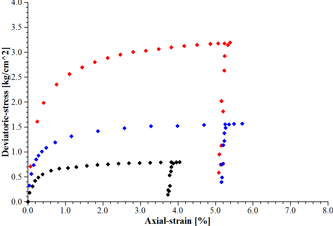
Figure 3: Original \(q\) vs. \(\varepsilon_1\) curves for the confining pressures of 1.2, 0.6, and 0.3 kgf/cm² of the triaxial compression tests of Monterey sand (Lade 1972).

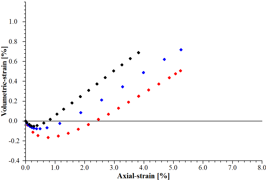
Figure 4: Original \(\varepsilon_v\) vs. \(\varepsilon_1\) curves for confining pressures of 1.2, 0.6, and 0.3 kgf/cm² of the triaxial compression tests of Monterey sand (Lade 1972).

break

Calibration of Friction Angle, \(\phi\), and Cohesion, \(c\):

The calibration of these two parameter has no difference from the Mohr-Coulomb model.

To estimate values of friction angle \(\phi\) and cohesion \(c\) from triaxial test data using the relation \(q = \sigma_3 - \sigma_1\) vs. \(p = -(\sigma_1 + 2\sigma_3)/3\), follow the procedure outlined below.

1. Plot deviatoric stress \(q\) vs. \(p\) using triaxial compression test lab data.
2. Use a trend line to fit the Mohr-Coulomb envelope.
3. The slope of the trend line is \(6 \sin \phi / (3 − \sin \phi)\), which follows from an alternative form of the Mohr-Coulomb failure criterion. This determines friction angle \(\phi\).
4. The intercept of the trend line is \(6c \cos \phi / (3 − \sin \phi)\), which determines cohesion \(c\), as the friction angle \(\phi\) is already known from the previous step.

Alternatively, these two parameters can be estimated from triaxial test data using the relation \(\hat{q} = (\sigma_3 - \sigma_1)/2\) vs. \(\hat{p} = -(\sigma_1 + \sigma_3)/2\) by following the procedure outlined below.

1. Plot deviatoric stress \(\hat{q}\) vs. \(\hat{p}\) using triaxial compression test lab data.
2. Use a trend line to fit the Mohr-Coulomb envelope.
3. The slope of the trend line is \(\sin \phi\), which follows from an alternative form of the Mohr-Coulomb failure criterion. This determines friction angle \(\phi\).
4. The intercept of the trend line is \(c \cos \phi\), which determines cohesion \(c\), as the friction angle \(\phi\) is already known from the previous step.

For the Monterey sand, the slope of the trend line of the Mohr-Coulomb envelope using the relation \(q\) vs. \(p\), presented in Figure 5, is 1.403. Based on this, the friction angle is calculated as 34.65 degrees. The intercept is approximately zero, which implies that the cohesion is zero.

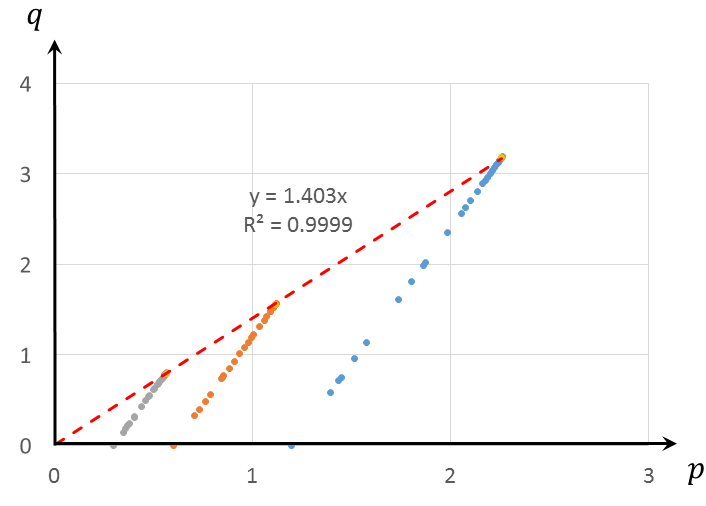
Figure 5: Determination of friction angle and cohesion from the triaxial compression test data.

Calibration of \(R_f\), \(m\), and \(E^{ref}_{50}\):

To estimate values of \(R_f\), \(m\), and \(E^{ref}_{50}\) from triaxial test data, follow the procedure outlined below.

1. Plot the curve of \(\varepsilon_1/q\) vs. \(\varepsilon_1/q_f\) using the triaxial compression test data.
2. Use a trend line to fit the data. The slope of the line is \(R_f\) , the intercept is \(1/E_i\), based on the relation \(\varepsilon_1/q = R_f (\varepsilon_1/q_f) + 1/E_i\) (derived from Equation (12) and \(R_f = q_f / q_a\)).

Multiple sets of triaxial compression tests with various confining pressures can be used to produce a set of pairs of (\(R_f\), \(E_{50}\)). The final \(R_f\) can be estimated as the averaged one, and the pairs of (\(E_i\), \(\sigma_3\)) determine \(m\) and \(E^{ref}_{50}\) based on Equation (7).

Figure 6 plots the curves of \(\varepsilon_1/q\) vs. \(\varepsilon_1/q_a\) using triaxial compression test data of the Monterey sand with confining pressures 1.2, 0.6, and 0.3 kgf/cm². The slopes of these lines are \(R_f\), and the intercepts are \(100/E_i\) (as strain is given in percentage).

This figure determines three pairs of (\(R_f\), \(E_{50}\)), summarized in Table 1. The average value for \(R_f\) is 0.957. Parameter \(p^{ref}\) needs no calibration and its value is assumed to be 0.1 kgf/cm². Finally, plotting parameters \(\ln (−\sigma_3/p^{ref})\) vs. \(\ln (E50)\), as shown in Figure 7, and using Equation (7) allows for determination of \(m\) and \(E^{ref}_{50}\) (remember that cohesion \(c\) = 0 for this example). The slope of the trend line in Figure 7 is \(m\) = 0.707 and the intercept determines \(E^{ref}_{50}\) = \(\exp{}\) (4.63) = 102.5 kgf/cm².

Table 1: Determination of \(R_f\), \(m\), and \(E^{ref}_{50}\)

\(\sigma_3\)	\(R_f\)	\(1/E_i\)	\(E_i\)	\(E_{50}\)	\(\ln (E_{50})\)	\(\ln \left( {c \cot \phi - \sigma_3} \over {c \cot \phi + p^{ref}} \right)\)
-0.3	0.9558	0.002459	406.7	212.3	5.358	1.099
-0.6	0.9678	0.001286	777.6	401.3	5.995	1.792
-1.2	0.9476	0.000930	1075.3	565.8	6.338	2.485

break

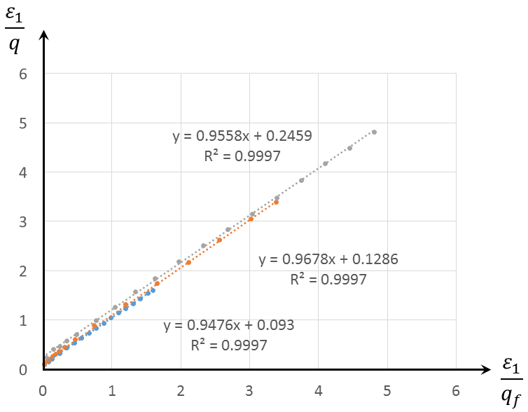
Figure 6: Determination of \(R_f\) and \(1/E_i\) from three sets of triaxial compression tests with three different confining stresses.

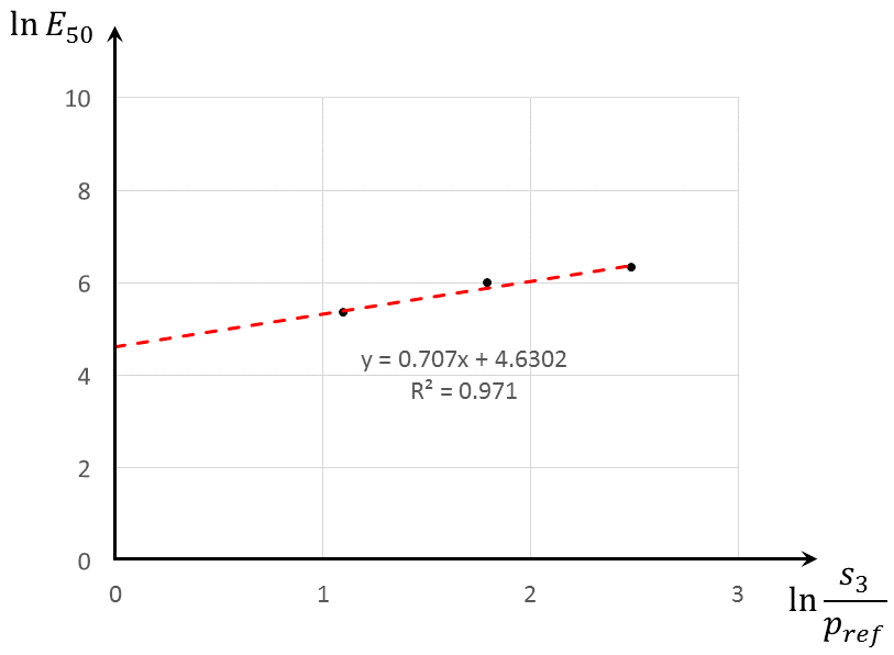
Figure 7: Determination of \(m\) and \(E^{ref}_{50}\) from three sets of triaxial compression tests with three different confining stresses.

break

Calibration of \(E^{ref}_{ur}\):

After the calibration of parameter \(m\), it is straightforward to obtain \(E^{ref}_{ur}\) from Equation (5) using the unloading-reloading modulus \(E_{ur}\) obtained from the original \(q\) vs. \(\varepsilon_1\) data in a triaxial compression test. The final value of \(E^{ref}_{ur}\) can be averaged using data for different confining pressures. For the example of Monterey sand, \(E^{ref}_{ur}\) is determined to be 320.0 kgf/cm². If the unloading-reloading moduli are not available, a value in the range of \((3 \sim 5) E^{ref}_{50}\) can be used for most soils. The PH model uses a default value of \(4 E^{ref}_{50}\) if no input is provided for \(E^{ref}_{ur}\).

Calibration of Dilation Angle, \(\psi\):

The ultimate dilation angle \(\psi\) can be estimated as \(\sin \psi = s_m / (s_m+2)\), where \(s_m\) is the maximum slope (\(s_m\)) of the \(\varepsilon_v\) vs. \(\varepsilon_1\) curve in the triaxial compression tests. The slope \(s_m\) is found as: \(s_m = -\Delta \varepsilon_v/\Delta \varepsilon_1 \approx -\Delta \varepsilon^p_v/\Delta \varepsilon^p_1 = 2\sin \psi/(1 - \sin \psi)\). For this example of the Monterey sand, the dilation angles are 6 ~ 7° (depending on confining pressure). The values are summarized in Table 2.

Calibration of \(K_{nc}\) and \(E^{ref}_{oed}\):

Parameters \(K_{nc}\) and \(E^{ref}_{oed}\) can be calibrated from the oedometer tests. The ultimate value of \(\sigma_3 / \sigma_1\) from an oedometer test is \(K_{nc}\). When \(\sigma_1 = -p^{ref}\), the tangent modulus of the \(\sigma_1\) vs. \(\varepsilon_1\) curve is \(E^{ref}_{oed}\).

Calibration of Poisson’s Ratio, \(\nu\):

Poisson’s ratio can be estimated from the initial slope \(s_0\) (usually a negative value) of the \(\varepsilon_v\) vs. \(\varepsilon_1\) curve, so that \(\nu = (1+\tan s_0)/2\). In the PH model, the default value is 0.2. In this example for Monetary Sand, the Poisson’s ratio is estimated to be 0.3.

Calibration of \(e_{max}\):

The material parameter \(e_{max}\) is needed if the dilation smoothing technique (Figure 2) is required. The value of \(e_{max}\) can be determined by conducting standard laboratory tests (ASTM D4254). If the standard ASTM D4254 laboratory test data are not available, its value can be estimated through the trial-and-error method based on the curves of the volumetric strain vs. axial strain of the triaxial compression tests. In this example, its value is estimated as 0.803. The default value of \(e_{max}\) = 999.0 is used when it is not provided as input, which implies that the dilation smoothing technique will not be activated.

Calibration of Other Parameters:

Such material parameters as \(\sigma^{ini}_1\), \(\sigma^{ini}_2\), \(\sigma^{ini}_3\), \(e_{ini}\), and \(OCR\) are known initial parameters and should be consistent with the initial conditions. Some parameters can be estimated through the trial-and-error method.

A summary of all material properties determined for the Monterey sand is provided in Table 2.

Table 2: Calibrated Material Parameters for Loose Monterey Sand

Parameters	\(\sigma_3\) = -1.2 (kgf/cm2)	\(\sigma_3\) = -0.6 (kgf/cm2)	\(\sigma_3\) = -0.3 (kgf/cm2)
\(E^{ref}_{50}\) (kgf/cm2)		102.5
\(E^{ref}_{ur}\) (kgf/cm2)		320.0
\(m\)		0.707
\(R_f\)		0.957
\(p^{ref}\) (kgf/cm2)		0.1
\(\nu\)		0.3
\(\phi\) (degrees)		34.65
\(c\) (kgf/cm2)		0.0
\(e_{max}\)		0.803
\(K_{nc}\)		0.5
\(\psi\) (degrees)	6.1	6.4	7.0
\(\sigma^{ini}_{1 \sim 3}\) (kgf/cm2)	-1.2	-0.6	-0.3
\(OCR\)	1.0	2.0	4.0
\(e_{ini}\)	0.783	0.786	0.781

Using these parameters, the triaxial compression tests can be simulated by the PH model. The plots presented in Figures 8 and 9 reveal a close match between the simulated results and laboratory test data.

break

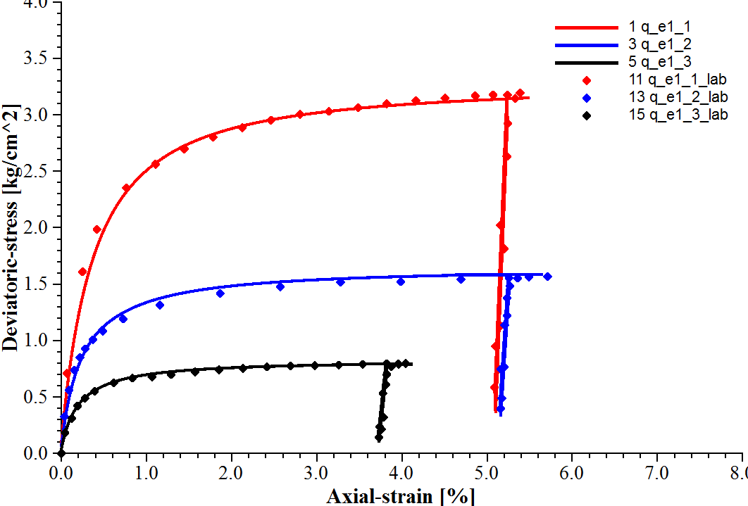
Figure 8: Deviatoric stress vs. axial strain for consolidated drained triaxial compression tests on fine Monterey sand.

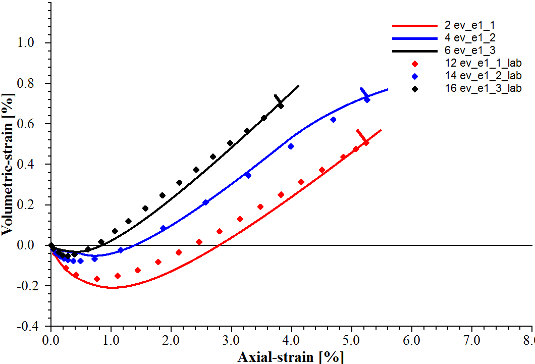
Figure 9: Volumetric strain vs. axial strain for consolidated drained triaxial compression tests on fine Monterey sand.

Small-Strain Stiffness Option

Using the Plastic-Hardening model to simulate the unloading-reloading paths, the reloading path will be the reverse of the unloading path. However, this elastic behavior assumes of very small strain. Experiments illustrate that soil stiffness modulus is strain-dependent – it decreases nonlinearly with the increase of shear strain. The strain can be categorized into three levels: the very small strain, where the stiffness modulus is assumed constant (\(G_0\) or sometimes called \(G_{max}\)); the small strain, where the stiffness modulus reduces non-linearly as the strain increases; and the large strain, where the soil is in or close to failure and the stiffness modulus is relatively small. Figures 10 illustrates this explanation using the normalized stiffness modulus degradation curve by comparing with the geotechnical applications and the measurement accuracy from the laboratory or in-situ tests. It is important that the soil stiffness modulus selected for simulation should not be associated to the strain levels at the end of the geotechnical constructions or from the laboratory tests with well disturbed samples, because the soil stiffness modulus could have decreased much from its initial value. The additional option of the small-strain stiffness modulus for the Plastic-Hardening model is objected to take the strain-dependency into account.

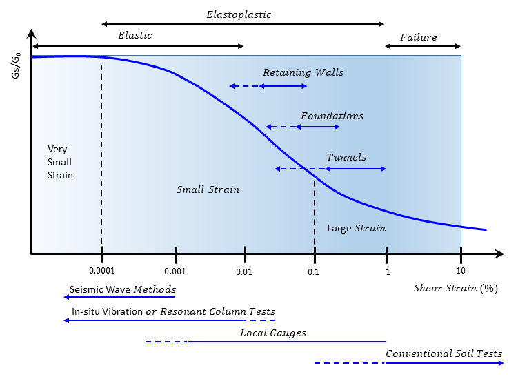
Figure 10: Stiffness modulus degradation curve and typical strain ranges (Modified from Atkinson and Sallfors 1991 and Ishihara 1996).

To activate the small-strain stiffness in Plastic-Hardening model, flag-smallstrain (the default is off) should be turned into on. Only two extra properties are required to be assigned: stiffness-0-reference (\(E_0^{ref}\)) and strain-70 (\(\gamma_{70}\)).

The initial stiffness modulus at the reference pressure, \(E_0^{ref}\), will determine the shear stiffness modulus (\(G_0\)) at the very small strain level. It can be estimated by the relations of

(40)\[E_0 = E_0^{ref} Z^m\]

and

(41)\[G_0 = \frac{E_0}{2(1+\nu)}\]

where \(Z\), \(m\) and \(\nu\) are defined in the standard Plastic-Hardening model. The default value of \(E_0^{ref}\) is taken as \(3 E_{ur}^{ref}\) if no specific data is available. \(E_0^{ref}\) is not allowed to be equal or smaller than \(E_{ur}^{ref}\) in this model. Together with the above two equations, \(E_0^{ref}\) could be estimated from

(42)\[G_0 = \rho V_s^2\]

where \(\rho\) is the soil density and \(V_s\) is the measured in-situ soil shear wave velocity. \(G_0\) can be estimated from other in-situ tests data, e.g., SPT, CPT & DMT, or from some accepted empirical relations.

The reference shear strain (\(\gamma_{70}\)) is selected the value at which the secant shear stiffness modulus is about 70% (accurately should be 72.2%) of \(G_0\). The default value for \(\gamma_{70}\) is 2e-4. Typical vales of \(\gamma_{70}\) is listed in Table 3:

Table 3: Typical vales of \(\gamma_{70}\)

Sand:
At depth 0 to 6 m	1.1e-4
At depth 6 to 15 m	1.6e-4
At depth 15 to 37 m	2.3e-4
At depth 37 to 76 m	3.3e-4
At depth 76 to 150 m	4.5e-4
At depth 150 to 300 m	7.0e-4
Clay:
Plastic Index = 30	3.5e-4
Plastic Index = 50	7.7e-4
Plastic Index = 100	1.8e-3

Once \(G_0\) and \(\gamma_{70}\) are known, the small-strain secant stiffness modulus is calculated as

(43)\[G_s = \frac{G_0}{1 + \frac{0.385\gamma}{\gamma_{70}}}\]

and its tangent stiffness modulus is

(44)\[G = \frac{G_0}{\left(1 + \frac{0.385\gamma}{\gamma_{70}}\right)^2}\]

The tangent shear stiffness modulus is setting a lower-bound value of \(G_{ur} = E_{ur} / [3(1-2\nu)]\) in this model.

The detailed algorithm to consider the unloading-reloading strain-dependent stiffness modulus is presented in Benz (2007). It should be noted that this algorithm may not preform well on nested hysteretic loops and is subjected to the so-called over-shooting problem. The plastic-Hardening model with small-strain stiffness is not recommended for fully dynamic problems with random unloading-reloading paths which leads to nested hysteretic loops.

References

Atkinson, J. H., & Sallfors, G. Experimental determination of stressstrain-time charactristics in laboratory and in situ tests. Proceedings, 10th ECSMFE, Florence, Rotterdam: Balkema, 959-999 (1991).

Benz, T. Small-strain stiffness of soils and its numerical consequences (Vol. 5). Stuttgart: Univ. Stuttgart, Inst. f. Geotechnik (2007).

Duncan, J. M., and C. Y. Chang. “Nonlinear Analysis of Stress and Strain in Soils,” Soil Mechanics, 96 (SM5), 1629-1653 (1970).

Ishihara, K. Soil behaviour in earthquake geotechnics. Clarendon Press (1996).

Schanz, T., Vermeer, P. A., & Bonnier, P. G. The hardening soil model: formulation and verification. Beyond 2000 in computational geotechnics, 281-296 (1999).

plastic-hardening Model Properties

Use the following keywords with the zone property command to set these properties of the plastic hardening model.

plastic-hardening

cohesion f

cohesion, \(c\). The default and cut-off (allowable minimum) value is \(10^{-5} \cdot p^{ref}\).

dilation f

ultimate dilation angle in degrees, \(\psi\). The default is 0.0.

exponent f

exponent for elastic moduli, \(m\). Allowable value is \(0 \le m \le 0.999\).

friction f

ultimate friction angle in degrees, \(\phi\). The default and cut-off (allowable minimum) value is 0.001 degrees.

stress-1-effective f

initial minimum principal effective stress, \(\sigma^{ini}_1\). See the note*.

stress-2-effective f

initial median principal effective stress, \(\sigma^{ini}_2\). See the note*.

stress-3-effective f

initial maximum principal effective stress, \(\sigma^{ini}_3\). See the note*.

pressure-reference f

reference pressure, \(p^{ref}\) . A non-zero value should be specified based on the unit of stress/pressure adopted in the model. Most commonly used and highly recommended reference pressure is the standard atmospheric pressure, e.g., 100.0 if in kPa, 1.0e5 if in Pa. or other value compatible to the adopted stress/pressure unit.

stiffness-50-reference f

secant stiffness, \(E^{ref}_{50}\), at 50% of the ultimate deviatoric stress, \(q_f\), when \(\sigma_3 = - p^{ref}\) in a triaxial test. A non-zero value must be specified.

stiffness-0-reference f

[advanced] Initial stiffness, \(E^{ref}_{0}\), at zero strain when \(\sigma_3 = - p^{ref}\). It is required that \(E^{ref}_{0} > E^{ref}_{ur}\). If not input or by default, \(E^{ref}_{0} = 3 \cdot E^{ref}_{ur}\). Need to be assigned only when the flag for small-strain stiffness is on, otherwise its value is useless.

stiffness-oedometer-reference f

[advanced] tangent stiffness, \(E^{ref}_{oed}\), when \(\sigma_1 = - p^{ref}\) in an oedometer test. By default, \(E^{ref}_{oed} = E^{ref}_{50}\) if \(E^{ref}_{oed}\) is not specified while \(E^{ref}_{50}\) has been specified.

stiffness-ur-reference f

[advanced] unloading-reloading stiffness, \(E^{ref}_{ur}\), when \(\sigma_3 = - p^{ref}\) in a triaxial test. This value must be greater than \(2 \cdot E^{ref}_{50}\). By default, \(E^{ref}_{ur} = 4 \cdot E^{ref}_{50}\).

coefficient-normally-consolidation f

[advanced] normal consolidation coefficient, \(K_{nc}\). It is not allowed to be less than \(\nu / (1-\nu)\), a range 0.5 to 0.7 is common. The default is \(K_{nc} = 1 - \sin \phi\).

constant-alpha f

[advanced] dimensionless parameter in the cap yield function, \(\alpha\). Initialized internally. See the note* for an alternative option.

factor-contraction f

[advanced] contraction factor, \(F_c\), allowable range is 0.0 to 0.25. The default is 0.0.

factor-cut f

[advanced] cut-off factor, \(f_{cut}\). The default is 0.1.

flag-initialization f

[advanced] flag for initialization. If set to 1, the internal variables will be recalculated. The default is 0.

flag-smallstrain f

[advanced] flag for small-strain stiffness . If set to on, the option of small-strain stiffness will be activated. The default is off.

over-consolidation-ratio f

[advanced] over consolidation ratio, \(OCR\). For normally consolidated soil, the value should be input as 1.0. The default is 100.0, which denotes an “apparent” non-cap shear plastic hardening model.

poisson f

[advanced] Poisson’s ratio, \(\nu\). The default is 0.2.

stiffness-cap-hardening f

[advanced] hardening modulus for cap hardening, \(H_c\). Initialized internally. See the note* for an alternative option.

strain-70 f

[advanced] Shear strain at which \(G_s / G_0\) = 72.2%, If not input or by default, \(\gamma_{70} = 2 \times 10^{-4}\). Need to be assigned only when the flag for small-strain stiffness is on, otherwise its value is useless.

failure-ratio f

[advanced] failure ratio, \(R_f\). The default is 0.9.

tension f

[advanced] tension limit, \(\sigma^t\). The default is 0.0.

void-initial f

[advanced] initial void ratio, \(e_{ini}\). If the current void ratio is not important, or you do not wish to activate the dilation smoothing technique, just use the default value. The default is 1.0.

void-maximum f

[advanced] allowable maximum void ratio, \(e_{max}\) . The default is 999.0, which is not physical but it denotes that the dilation smoothing technical will nominally not activated.

bulk f

[read only] current loading-unloading bulk modulus, \(K\)

shear f

[read only] current unloading-reloading shear modulus, \(G\)

plastic-hardening-shear f

[read only] accumulated shear plastic hardening parameter, \(\gamma^p\)

plastic-hardening-volume f

[read only] accumulated volumetric plastic hardening parameter, \(\varepsilon^p_v\)

pressure-cap f

[read only] cap (preconsolidation) pressure, \(p_c\). Determined by the current stress, \(\alpha\), and \(OCR\).

void f

[read only] current void ratio, \(e\)

Notes:

• The tension cut-off is \({\sigma}^t = min({\sigma}^t, c/\tan \phi)\).
• The parameters \(\sigma^{ini}_1\), \(\sigma^{ini}_2\), \(\sigma^{ini}_3\) must be specified via commands or a FISH function the first time the PH model is assigned because it is a stress-dependent model. Negative values denote compressive stresses.
• Some parameter combinations may be rejected due to: 1) one or more parameters are out of predetermined limits; 2) internal parameters cannot be correctly determined; or 3) numerical instability.
• If both \(\alpha\) and \(H_c\) are specified non-zero values by the user, the PH model will use these user-defined parameters \(\alpha\) and \(H_c\), and the internal calculation for \(\alpha\) and \(H_c\) will not be performed.

Footnotes

Advanced properties have default values and do not require specification for simpler applications of the model.

Read only properties cannot be set by the user. However, they may be listed, plotted, or accessed through FISH.