FLAC3D Theory and Background • Constitutive Models

Ubiquitous-Joint Model

This model accounts for the presence of an orientation of weakness (weak plane) in a FLAC3D Mohr-Coulomb model. The criterion for failure on the plane, whose orientation is given, consists of a composite Mohr-Coulomb envelope with tension cutoff. The position of a stress point on the latter envelope is controlled again by a nonassociated flow rule for shear failure and an associated rule for tension failure.

In this numerical model, general failure is first detected and relevant plastic corrections are applied, as indicated in the FLAC3D Mohr-Coulomb model description. The new stresses are then analyzed for failure on the weak plane and updated accordingly. The FLAC3D Mohr-Coulomb model was addressed earlier; developments related to plastic flow on the weak plane will be discussed in this section.

Definitions

The weak-plane orientation is given by the Cartesian components of a unit normal to the plane in the global $x$-, $y$-, $z$-axes. A local system of reference axes is defined with $x'$ and $y'$ in the plane and $z'$ pointing in the direction of the unit normal $[n]$. (The $x'$-axis points downward in the dip direction, and the $y'$-axis is horizontal. The local system is right-handed.)

Using a matrix notation, we define $[C]$ as the rotation tensor whose three columns are the direction cosines of $x'$, $y'$, and $[n]$. The stress components in the local axes ${\sigma}_{i'j'}$ are computed using the transformation

(1) $$[\sigma]' = [C]^T [\sigma] [C]$$

In turn, the global stress components may be obtained from the local components using the reverse transformation,

(2) $$[\sigma] = [C] [\sigma]' [C]^T$$

The magnitude of the tangential traction component on the weak plane, referred to as $\tau$, is defined as

(3) $$\tau = \sqrt{{{\sigma}_{1'3'}}^2 + {{\sigma}_{2'3'}}^2}$$

The strain variable associated with $\tau$ is $\gamma$ and has the form

(4) $$\gamma = \sqrt{{{\epsilon}_{1'3'}}^2 + {{\epsilon}_{2'3'}}^2}$$

In what follows, we use ${\sigma}_{ij}^O$ to refer to the stress components obtained at the end of the current timestep, after application of the plastic corrections related to general failure only (as opposed to failure on the weak plane).

Weak-Plane Generalized Stress and Strain Components

The generalized stress vector used to describe weak-plane failure has four components ($n$ = 4): ${\sigma}_{1'1'}$, ${\sigma}_{2'2'}$, ${\sigma}_{3'3'}$, and $\tau$. The components of the corresponding generalized strain vector are ${\epsilon}_{1'1'}$, ${\epsilon}_{2'2'}$, ${\epsilon}_{3'3'}$, and $\gamma$.

Incremental Elastic Law

The incremental expression of Hooke’s law in terms of the generalized stress and strain increments has the form (see Elastic Model)

(5) $$\begin{split}\begin{matrix} \Delta {\sigma}_{1'1'} = {\alpha}_1 \Delta {\epsilon}_{1'1'}^e + {\alpha}_2 (\Delta {\epsilon}_{2'2'}^e + \Delta {\epsilon}_{3'3'}^e) \\ \\ \Delta {\sigma}_{2'2'} = {\alpha}_1 \Delta {\epsilon}_{2'2'}^e + {\alpha}_2 (\Delta {\epsilon}_{1'1'}^e + \Delta {\epsilon}_{3'3'}^e) \\ \\ \Delta {\sigma}_{3'3'} = {\alpha}_1 \Delta {\epsilon}_{3'3'}^e + {\alpha}_2 (\Delta {\epsilon}_{1'1'}^e + \Delta {\epsilon}_{2'2'}^e) \\ \\ \Delta \tau = 2G \Delta {\gamma}^e \end{matrix}\end{split}$$

where ${\alpha}_1$ and ${\alpha}_2$ are material constants defined in terms of the shear modulus, $G$, and bulk modulus, $K$, as

(6) $$\begin{split}\begin{matrix} {\alpha}_1 = K + {{4}\over{3}} G \\ \\ {\alpha}_2 = K - {{2}\over{3}} G \end{matrix}\end{split}$$

For future reference, comparing those expressions on $S_i$ in Incremental Formula:

(7) $$\begin{split}\begin{matrix} S_1(\Delta {\epsilon}_{1'1'}^e,\Delta {\epsilon}_{2'2'}^e,\Delta {\epsilon}_{3'3'}^e, \Delta {\gamma}^e) = {\alpha}_1 \Delta {\epsilon}_{1'1'}^e + {\alpha}_2 (\Delta {\epsilon}_{2'2'}^e + \Delta {\epsilon}_{3'3'}^e) \\ \\ S_2(\Delta {\epsilon}_{1'1'}^e,\Delta {\epsilon}_{2'2'}^e,\Delta {\epsilon}_{3'3'}^e,\Delta {\gamma}^e) = {\alpha}_1 \Delta {\epsilon}_{2'2'}^e + {\alpha}_2 (\Delta {\epsilon}_{1'1'}^e + \Delta {\epsilon}_{3'3'}^e) \\ \\ S_3(\Delta {\epsilon}_{1'1'}^e,\Delta {\epsilon}_{2'2'}^e,\Delta {\epsilon}_{3'3'}^e,\Delta {\gamma}^e) = {\alpha}_1 \Delta {\epsilon}_{3'3'}^e + {\alpha}_2 (\Delta {\epsilon}_{1'1'}^e + \Delta {\epsilon}_{2'2'}^e) \\ \\ S_4(\Delta {\epsilon}_{1'1'}^e,\Delta {\epsilon}_{2'2'}^e,\Delta {\epsilon}_{3'3'}^e, \Delta {\gamma}^e) = 2G \Delta {\gamma}^e \end{matrix}\end{split}$$

Note that the elastic strain increments in the preceding formula may be expressed as differences between total and plastic strain increments. Taking into consideration that the plastic increments may contain a known contribution associated with general failure (as opposed to weak plane failure), the derivation leading to the expressions for the new stresses may be followed (see Incremental Formulation), provided we interpret ${\underline{\sigma}}_i^I$ as the generalized stress component, ${\underline{\sigma}}_i^O$, obtained at the end of the current timestep, after application of the plastic corrections relating to general failure only.

Composite Failure Criterion and Flow Rule

The weak-plane failure criterion used in the FLAC3D model is a composite Mohr-Coulomb criterion with tension cutoff expressed in terms of (${\sigma}_{3'3'}$, $\tau$), as illustrated in Figure 1. (Recall that compressive stresses are negative.) The failure envelope $f({\sigma}_{3'3'},\tau) = 0$ is defined from point $A$ to $B$ by the Mohr-Coulomb failure criterion $f^s$ = 0, with

(8) $$f^s = \tau + {\sigma}_{3'3'} \ \tan {\phi}_j - c_j$$

and from $B$ to $C$ by a tension failure criterion of the form $f^t$ = 0, with

(9) $$f^t = {\sigma}_{3'3'} - {\sigma}_j^t$$

where ${\phi}_j$, $c_j$, and ${\sigma}_j^t$ are the friction, cohesion, and tensile strength of the weak plane, respectively. Note that for a weak plane with nonzero friction angle, the maximum value of the tensile strength is given by

(10) $${{\sigma}_j^t}_{max} = {{c_j}\over{\tan {\phi}_j}}$$

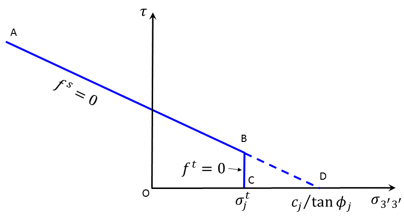
Figure 1: FLAC3D weak-plane failure criterion.

The potential function is composed of two functions ($g^s$ and $g^t$) used to define shear and tensile plastic flow, respectively. The function $g^s$ corresponds to a nonassociated law and has the form

(11) $$g^s = \tau + {\sigma}_{3'3'} \tan {\psi}_j$$

where $\psi$ is the weak-plane dilation angle. The function $g^t$ corresponds to an associated flow rule and is written as

(12) $$g^t = {\sigma}_{3'3'}$$

An elastic guess violating the composite yield function is represented by a point in the $({\sigma}_{3'3'},\tau)$-plane located either in domain 1 or 2, partitioned by the diagonal line between the lines defined by $f^s=0$ and $f^t=0$ (see Figure 2). If in domain 1, shear failure is declared and the stress point is placed on the curve $f^s$ = 0 using a flow rule derived using the potential function $g^s$. If in domain 2, tensile failure takes place and the stress point conforms to $f^t$ = 0 using a flow rule derived using $g^t$.

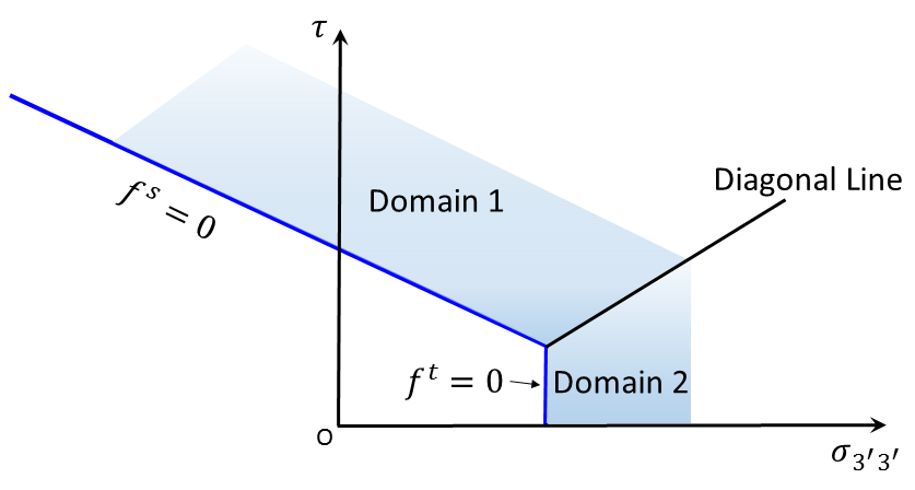
Figure 2: Ubiquitous-joint model—domains used in the definition of the weak-plane flow rule.

Plastic Corrections

First, considering shear failure (domain 1), partial differentiation of Equation (8) yields

(13) $$\begin{split}\begin{matrix} {{\partial g^s}\over{\partial {\sigma}_{1'1'}}} = 0 \\ \\ {{\partial g^s}\over{\partial {\sigma}_{2'2'}}} = 0 \\ \\ {{\partial g^s}\over{\partial {\sigma}_{3'3'}}} = \tan {\psi}_j \\ \\ {{\partial g^s}\over{\partial \tau}} = 1 \end{matrix}\end{split}$$

Substitution of $\partial g^s / \partial {\sigma}_{1'1'}$, $\partial g^s / \partial {\sigma}_{2'2'}$, $\partial g^s / \partial {\sigma}_{3'3'}$, and $\partial g^s / \partial \tau$ for $\Delta {\epsilon}_{1'1'}^e$, $\Delta {\epsilon}_{2'2'}^e$, $\Delta {\epsilon}_{3'3'}^e$, and $\Delta {\gamma}^e$, respectively, in Equation (7), gives

(14) $$\begin{split}\begin{matrix} S_1({{\partial g^s}\over{\partial {\sigma}_{1'1'}}}, {{\partial g^s}\over{\partial {\sigma}_{2'2'}}}, {{\partial g^s}\over{\partial {\sigma}_{3'3'}}}, {{\partial g^s}\over{\partial \tau}}) = {\alpha}_2 \tan {\psi}_j \\ \\ S_2({{\partial g^s}\over{\partial {\sigma}_{1'1'}}}, {{\partial g^s}\over{\partial {\sigma}_{2'2'}}}, {{\partial g^s}\over{\partial {\sigma}_{3'3'}}}, {{\partial g^s}\over{\partial \tau}}) = {\alpha}_2 \tan {\psi}_j \\ \\ S_3({{\partial g^s}\over{\partial {\sigma}_{1'1'}}}, {{\partial g^s}\over{\partial {\sigma}_{2'2'}}}, {{\partial g^s}\over{\partial {\sigma}_{3'3'}}}, {{\partial g^s}\over{\partial \tau}}) = {\alpha}_1 \tan {\psi}_j \\ \\ S_4({{\partial g^s}\over{\partial {\sigma}_{1'1'}}}, {{\partial g^s}\over{\partial {\sigma}_{2'2'}}}, {{\partial g^s}\over{\partial {\sigma}_{3'3'}}}, {{\partial g^s}\over{\partial \tau}}) = 2G \end{matrix}\end{split}$$

Using $f = f^s$ (see Equation (8)):

(15) $$\begin{split}\begin{matrix} {\sigma}_{1'1'}^N = {\sigma}_{1'1'}^O - {\lambda}^s {\alpha}_2 \tan {\psi}_j \\ \\ {\sigma}_{2'2'}^N = {\sigma}_{2'2'}^O - {\lambda}^s {\alpha}_2 \tan {\psi}_j \\ \\ {\sigma}_{3'3'}^N = {\sigma}_{3'3'}^O - {\lambda}^s {\alpha}_1 \tan {\psi}_j \end{matrix}\end{split}$$

(16) $${\tau}^N = {\tau}^O - {\lambda}^s 2G$$

and

(17) $${\lambda}^s = {{f^s ({\sigma}_{3'3'}^O,{\tau}^O)}\over{2G + {\alpha}_1 \tan {\psi}_j \tan {\phi}_j}}$$

The new shear stress components on the weak plane may be derived from ${\tau}^N$ and ${\tau}^O$, using the relations

(18) $$\begin{split}\begin{matrix} {\sigma}_{1'3'}^N = {\sigma}_{1'3'}^O {{{\tau}^N}\over{{\tau}^O}} \\ \\ {\sigma}_{2'3'}^N = {\sigma}_{2'3'}^O {{{\tau}^N}\over{{\tau}^O}} \\ \end{matrix}\end{split}$$

The stress corrections for shear failure may thus be expressed as (see Equation (15) and Equation (18))

(19) $$\begin{split}\begin{matrix} \Delta {\sigma}_{1'1'} = - {\lambda}^s {\alpha}_2 \tan {\psi}_j \\ \\ \Delta {\sigma}_{2'2'} = - {\lambda}^s {\alpha}_2 \tan {\psi}_j \\ \\ \Delta {\sigma}_{3'3'} = - {\lambda}^s {\alpha}_1 \tan {\psi}_j \\ \\ \Delta {\sigma}_{1'3'} = {\sigma}_{1'3'}^O {{{\tau}^N - {\tau}^O}\over{{\tau}^O}} \\ \\ \Delta {\sigma}_{2'3'} = {\sigma}_{2'3'}^O {{{\tau}^N - {\tau}^O}\over{{\tau}^O}} \end{matrix}\end{split}$$

We now consider tensile failure (domain 2). Partial differentiation of Equation (9) gives

(20) $$\begin{split}\begin{matrix} {{\partial g^t}\over{\partial {\sigma}_{1'1'}}} = 0 \\ \\ {{\partial g^t}\over{\partial {\sigma}_{2'2'}}} = 0 \\ \\ {{\partial g^t}\over{\partial {\sigma}_{3'3'}}} = 1 \\ \\ {{\partial g^t}\over{\partial \tau}} = 0 \end{matrix}\end{split}$$

Using Equation (14), we obtain

(21) $$\begin{split}\begin{matrix} S_1({{\partial g^t}\over{\partial {\sigma}_{1'1'}}}, {{\partial g^t}\over{\partial {\sigma}_{2'2'}}}, {{\partial g^t}\over{\partial {\sigma}_{3'3'}}}, {{\partial g^t}\over{\partial \tau}}) = {\alpha}_2 \\ \\ S_2({{\partial g^t}\over{\partial {\sigma}_{1'1'}}}, {{\partial g^t}\over{\partial {\sigma}_{2'2'}}}, {{\partial g^t}\over{\partial {\sigma}_{3'3'}}}, {{\partial g^t}\over{\partial \tau}}) = {\alpha}_2 \\ \\ S_3({{\partial g^t}\over{\partial {\sigma}_{1'1'}}}, {{\partial g^t}\over{\partial {\sigma}_{2'2'}}}, {{\partial g^t}\over{\partial {\sigma}_{3'3'}}}, {{\partial g^t}\over{\partial \tau}}) = {\alpha}_1 \\ \\ S_4({{\partial g^t}\over{\partial {\sigma}_{1'1'}}}, {{\partial g^t}\over{\partial {\sigma}_{2'2'}}}, {{\partial g^t}\over{\partial {\sigma}_{3'3'}}}, {{\partial g^t}\over{\partial \tau}}) = 0 \end{matrix}\end{split}$$

With $f = f^t$ as given by Equation (9):

(22) $$\begin{split}\begin{matrix} {\sigma}_{1'1'}^N = {\sigma}_{1'1'}^O - {\lambda}^t {\alpha}_2 \\ \\ {\sigma}_{2'2'}^N = {\sigma}_{2'2'}^O - {\lambda}^t {\alpha}_2 \\ \\ {\sigma}_{3'3'}^N = {\sigma}_{3'3'}^O - {\lambda}^t {\alpha}_1 \end{matrix}\end{split}$$

and

(23) $${\lambda}^t = {{{\sigma}_{3'3'}^O - {\sigma}_j^t}\over{{\alpha}_1}}$$

Finally, the stress corrections for tensile failure may be expressed, after substitution of Equation (23) for ${\lambda}^t$ in Equation (22), in the form

(24) $$\begin{split}\begin{matrix} \Delta {\sigma}_{1'1'} = - ({\sigma}_{3'3'}^O - {\sigma}_j^t) {{{\alpha}_2}\over{{\alpha}_1}} \\ \\ \Delta {\sigma}_{2'2'} = - ({\sigma}_{3'3'}^O - {\sigma}_j^t) {{{\alpha}_2}\over{{\alpha}_1}} \\ \\ \Delta {\sigma}_{3'3'} = {\sigma}_j^t - {\sigma}_{3'3'}^O \end{matrix}\end{split}$$

Large-Strain Update to Orientation

In large strain, the orientation of the weak plane is adjusted, per zone, to account for rigid-body rotations and rotations due to deformations. The corrections applied to the global components of the unit normal to the weak plane are computed, at each step, as averages over all tetra involved in the zone.

First taking into account rotations due to deformations, the corrections in local axes $\Delta [n]'^d$ to the weak-plane normal may be expressed as

(25) $$\begin{split}\begin{matrix} \Delta n_{1'}^d = - \Delta {\epsilon}_{1'3'} \\ \\ \Delta n_{2'}^d = - \Delta {\epsilon}_{2'3'} \\ \\ \Delta n_{3'}^d = 0 \end{matrix}\end{split}$$

The corresponding global components $\Delta n_1^d, \Delta n_2^d, \Delta n_3^d$ are obtained using the transformation

(26) $$\Delta [n]^d = [C] \Delta [n]'^d$$

where $[C]$ is the rotation tensor introduced above.

In turn, rigid-body rotations are taken into consideration by application of the rotation tensor $[\omega] + [I]$ to $\Delta [n]^d$, where $[I]$ is the identity matrix, and $[\omega]$ is defined in Rate of Strain and Rate of Rotation (see ${\omega}_{ij}$). In further neglecting second-order terms, the total corrections to be added to $[n]$ to obtain the new value $[n]^N$ have the form

(27) $$\Delta [n]^N = [\omega] [n] + \Delta [n]^d$$

Apex Stress Correction

It is possible that $\sigma_{3'3'}$ is greater than the apex stress ($c_j/\tan {\phi_j}$) at an extreme circumstance when $\phi_j$ is not zero (usually after shear plastic corrections). Once this occurs, the stress will be forced to the apex, or $\sigma_{3'3'} = c_j/\tan {\phi_j}$ and $\tau=0$.

Implementation Procedure

In the implementation of the ubiquitous-joint model in FLAC3D, stresses corresponding to the elastic guess for the step are first analyzed for general failure, and relevant plastic corrections are made, as described in the FLAC3D Mohr-Coulomb model. The resulting stress components, labeled as ${\sigma}_{ij}^O$, are then examined for failure on the weak plane.

Local stress components ${\sigma}_{1'1'}^O, {\sigma}_{2'2'}^O, {\sigma}_{3'3'}^O$ and ${\tau}^O$ are first evaluated using the transformation Equation (1) and the expression Equation (3). Following sentence is incomplete. If the stresses ${\sigma}_{3'3'}^O$ and ${\tau}^O$ violate the composite yield criterion (see Equation (8) and Equation (9)), then either in domain 1 (shear failure) or domain 2 (tension failure). In the first case, shear failure takes place, and the stress corrections $\Delta {\sigma}_{1'1'}$, $\Delta {\sigma}_{2'2'}$, $\Delta {\sigma}_{3'3'}$, $\Delta {\sigma}_{1'3'}$, and $\Delta {\sigma}_{2'3'}$ are evaluated from Equation (14), using Equation (17). In the second case, tensile failure occurs and the stress corrections $\Delta {\sigma}_{1'1'}$, $\Delta {\sigma}_{2'2'}$, and $\Delta {\sigma}_{3'3'}$ are evaluated from Equation (24), using Equation (23). The tensor of stress corrections is expressed in the system of reference axes using the transformation of Equation (2) and added to $[\sigma]^O$ to yield new stress values.

If the point $({\sigma}_{3'3'}^O, {\tau}^O)$ is located below the representation of the composite failure envelope in the plane $({\sigma}_{3'3'}, \tau)$, no plastic flow takes place for this step, and the new stresses are given by ${\sigma}_{ij}^O$.

In large-strain mode, the unit normal to the weak plane is adjusted per zone to account for body rotations (see Equation (25) and Equation (26)).

Note that the default value for the weak-plane tensile strength is zero if ${\phi}_j$ = 0, and ${{\sigma}_j^t}_{max}$ otherwise (see Equation (10)). This last value is substituted for ${{\sigma}^t}$ if the value assigned for the weak plane tensile strength exceeds ${{\sigma}_j^t}_{max}$.

ubiquitous-joint Model Properties

Use the following keywords with the zone property command to set these properties of the ubiquitous-joint model.

ubiquitous-joint

bulk f

elastic bulk modulus, $K$

cohesion f

cohesion, $c$

dilation f

dilation angle, $\psi$. The default is 0.0.

dip f

dip angle [degrees] of weakness plane

dip-direction f

dip direction [degrees] of weakness plane

friction f

internal angle of friction, $\phi$

poisson f

Poisson’s ratio, $\nu$

shear f

elastic shear modulus, $G$

tension f

tension limit, ${\sigma}^t$. The default is 0.0.

young f

Young’s modulus, $E$

joint-cohesion f

joint cohesion, $c_j$

joint-dilation f

joint dilation angle, ${\psi}_j$. The default is 0.0.

joint-friction f

joint friction angle, ${\phi}_j$

joint-tension f

joint tension limit, ${\sigma}^t_j$. The default is 0.0.

normal v

normal direction of the weakness plane, ($n_x$, $n_y$, $n_z$)

normal-x f

x-component of the normal direction to the weakness plane, $n_x$

normal-y f

y-component of the normal direction to the weakness plane, $n_y$

normal-z f

z-component of the normal direction to the weakness plane, $n_z$

flag-brittle b

[advanced] If true, the tension limit is set to 0 in the event of tensile failure. The default is false.

Notes:

• Only one of the two options is required to define the elasticity: bulk modulus $K$ and shear modulus $G$, or, Young’s modulus $E$ and Poisson’s ratio $\nu$. When choosing the latter, Young’s modulus $E$ must be assigned in advance of Poisson’s ratio $\nu$.
• Only one of the three options is required to define the orientation of the weakness plane: dip and dip-direction; a norm vector ($n_x, n_y, n_z$); or, three norm components: $n_x$, $n_y$, and $n_z$.
• The tension cut-off is ${\sigma}^t = min({\sigma}^t, c/\tan \phi)$.
• The joint tension limit used in the model is the minimum of the input $\sigma^t$ and ${c_j}/{\tan \phi_j}$.

Footnote

Advanced properties have default values and do not require specification for simpler applications of the model.