Loading and Sequential Modeling
By applying different model loading conditions at different stages of an analysis, it is possible to simulate changes in physical loading, such as sequences of excavation and construction. Changes in loading may be specified in a number of ways (e.g., by applying new stress or displacement boundaries, by changing the material model in zones to either a null material or to a different material model, or by changing material properties).
It is important to recognize that sequential modeling follows the stages of an engineering work (e.g., the stages in excavation and construction of a sheet pile wall). This modeling does not, however, include physical time as a parameter, and time-dependent behavior cannot be simulated.[1] Some engineering judgment must be used to estimate the effects of time. For example, a model parameter may be changed after a predetermined amount of displacement or strain has occurred. This displacement may be estimated to have occurred over a given period of time.
The following guidelines should be followed when performing loading changes or defining stages in a sequential analysis:
- As discussed in the Grid Generation section, all regions to be excavated must correspond to zone boundaries established on creation. Zones and gridpoints can be moved after creation, but their stress states will not adjust to the new configuration, stresses are only modified as a result of velocity increments during cycling.
- Zones and gridpoints can be created after cycling, to add material to a dam for example. But these zones are created with zero stresses and no constitutive model, as with all zones on creation.
- In general, excavations should use
zone relax excavateto minimize pseudo-inertial effects on the solution.- When material models are changed during a simulation sequence, all properties must be re-specified for the new model, even if the affected zones were previously assigned the same properties. Properties are lost when models are changed. Stresses in zones are preserved when models are changed, unless the zones are changed to null zones; in this case, all stresses in the affected zones are set to zero.
- If the model is in equilibrium, a change in elastic properties will have no effect on the response of the model because elastic moduli are tangent moduli, not secant moduli. The model must be subjected to a change that causes unbalanced forces to develop. This may be caused, for example, by a change in strength properties if the current stresses exceed the new strength limit.
The recommended approach to sequential modeling is demonstrated in the example that follows this topic.
Example: Loading on Three Tunnels
This problem involves the analysis of the loading on three tunnels (a service tunnel and two main tunnels) that are sequentially excavated and lined. The grid generation for this problem was described previously in Fitting the Grid to Simple Shapes.
The construction sequence to be analyzed consists of three modeling stages:
- excavation of the first half of a service tunnel; then
- installation of a liner in the first half, and excavation of the second half of the service tunnel; then
- installation of the liner in the second half of the service tunnel, and excavation of the first half of the main tunnel.
The objective of the analysis is to investigate the influence of the main tunnel excavation on the response of the service tunnel.
The model is constructed to take advantage of symmetry in the problem. The service tunnel is located midway between the main tunnels, so a vertical plane of symmetry may be assumed to exist along the centerline of the service tunnel. The model grid is created in the following data file.
Sequential excavation and lining of tunnels — initial grid
model new
model largestrain off
; main tunnel
zone create radial-cylinder point 0 (15, 0,0) point 1 (23,0,0) ...
                            point 2 (15,50,0) point 3 (15,0,8) ...
                            size 4 10 6 4 dim 4 4 4 4 rat 1 1 1 1 ...
                            group 'rock' fill group 'main1'
zone reflect dip 90 dip-direction 90 origin (15,0,0)
zone reflect dip 0 origin (0,0,0)
; service tunnel - create two gridpoints as reference location
zone gridpoint create (2.969848, 0.0,-0.575736) name='ref1'
zone gridpoint create (2.969848,50.0,-0.575736) name='ref2'
zone create radial-cylinder point 0 (0, 0,-1) point 1 (7, 0,0) ...
                            point 2 (0,50,-1) point 3 (0, 0,8) ...
                            point 4 (7,50, 0) point 5 (0,50,8) ...
                            point 6 (7, 0, 8) point 7 (7,50,8) ...
                            point 8 gridpoint 'ref1' point 10 gridpoint 'ref2' ...
                            size 3 10 6 4 dim 3 3 3 3 rat 1 1 1 1 ...
                            group 'rock' fill group 'service1'
zone create radial-cylinder point 0 (0, 0,-1) point 1 (0, 0,-8) ...
                            point 2 (0,50,-1) point 3 (7, 0, 0) ...
                            point 4 (0,50,-8) point 5 (7,50, 0) ...
                            point 6 (7, 0,-8) point 7 (7,50,-8) ...
                            point 9 gridpoint 'ref1' point 11 gridpoint 'ref2' ...
                            size 3 10 6 4 dim 3 3 3 3 rat 1 1 1 1 ...
                            group 'rock' fill group 'service1'
; outer boundary
zone create radial-tunnel point  0 ( 7, 0, 0) point  1 (50, 0, 0) ...
                          point  2 ( 7,50, 0) point  3 (15, 0,50) ...
                          point  4 (50,50, 0) point  5 (15,50,50) ...
                          point  6 (50, 0,50) point  7 (50,50,50) ...
                          point  8 (23, 0, 0) point  9 ( 7, 0, 8) ...
                          point 10 (23,50, 0) point 11 ( 7,50, 8) ...
                          size 6 10 3 10 rat 1 1 1 1.1 group 'rock'
zone create brick point 0 ( 0,0, 8) point 1 ( 7, 0, 8) point 2 (0,50, 8) ...
                  point 3 ( 0,0,50) point 4 ( 7,50, 8) point 5 (0,50,50) ...
                  point 6 (15,0,50) point 7 (15,50,50) ...
                  size 3 10 10 rat 1 1 1.1 group 'rock'
zone reflect dip 0 origin (0,0,0) range position-x  0 23 position-y 0 50 position-z 8 50
zone reflect dip 0 origin (0,0,0) range position-x 23 50 position-y 0 50 position-z 0 50
zone group 'main2' range group 'main1' position-y 25 50
zone group 'service2' range group 'service1' position-y 25 50
zone face group 'liner1' internal range group 'service1' group 'rock'
zone face group 'liner2' internal range group 'service2' group 'rock'
zone face skin
model save 'grid'
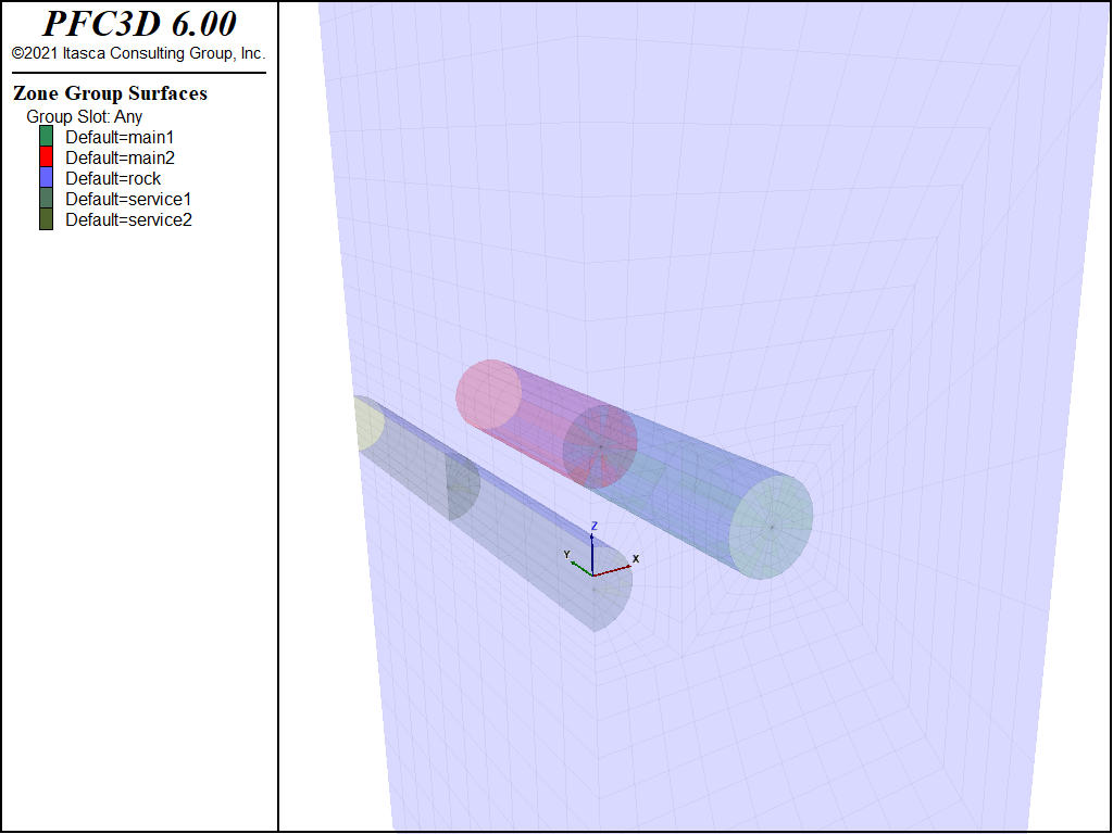
The resulting grid is shown in the next figure. The grid is manipulated such that the invert of the service tunnel is at the same elevation as that of the main tunnel (see Fitting the Grid to Simple Shapes).
A Mohr-Coulomb material model is initially defined for all zones. The plane of symmetry is specified, and an isotropic initial stress is assigned to the model. The model is in force equilibrium before an excavation is made. Note that only one calculation step is taken when the model solve command is issued, because the model is in equilibrium for the specified boundary and initial conditions. The next listing shows the commands for this stage.
Sequential excavation and lining of tunnels — initial state
model restore 'grid'
; mohr-coulomb model
zone cmodel assign mohr-coulomb
zone property shear 0.36e9 bulk 0.6e9 cohesion 1e5 friction 20 tension 1e5
; Boundary conditions
zone face apply velocity-normal 0 range group 'Bottom'
zone face apply velocity-normal 0 range group 'East' or 'West'
zone face apply velocity-normal 0 range group 'North' or 'South'
zone face apply stress-normal -1.4e6 range group 'Top'
; Initial Conditions
zone initialize stress xx -1.4e6 yy -1.4e6 zz -1.4e6
; Histories
model history name='conv' mechanical convergence
zone history name='s-f' displacement-x position (3,0,-1)
zone history name='c-f' displacement-z position (0,0,2)
zone history name='s-m' displacement-x position (3,25,-1)
zone history name='c-m' displacement-z position (0,25,2)
model solve convergence 1
model save 'initial'
In the first stage, the solution is found with a 25 m section of the service tunnel excavated. The excavation is made using the zone relax excavate command. [2] The stage 1 commands are listed below.
Sequential excavation and lining of tunnels — stage 1
; exacavate 25 m section of service tunnel
model restore 'initial'
zone relax excavate range group 'service1'
model solve convergence 1
model save 'stage1'
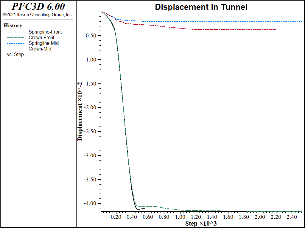
The gridpoint history plots in the next figure for displacement at the springline and crown of the service tunnel indicate that the model has reached equilibrium within approximately 2500 calculation steps for stage 1.
In the second stage, the lining is installed along the excavated section of the service tunnel. The lining is modeled using structural shell elements, and an elastic liner is assumed. Fixity conditions are specified for structural element nodes located on the symmetry plane of the grid to correspond to the same symmetry condition for the liner.
The second 25 m section of the service tunnel is then excavated, and the solution is calculated for support provided by the lining, as seen here:
Sequential excavation and lining of tunnels — stage 2
model restore 'stage1'
zone gridpoint initialize displacement (0,0,0)
history purge
; Excavate second half of service tunnel
zone relax excavate range group 'service2'
; Install liner in first half of service tunnel
struct shell create by-face range group 'liner1'
struct shell property isotropic (25.3e9,0.266) thick 0.5
; Shell symmetry boundary conditions
struct node fix velocity-y rotation-x rotation-z range position-y 0
struct node fix velocity-x rotation-y rotation-z range position-x 0
; Solve to equilibrium
model solve convergence 1
model save 'stage2'
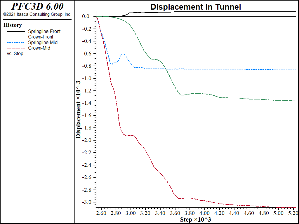
We initialize the displacements in the model so that we can focus on the response due only to the excavation in the second stage. The displacement histories at the two ends of the lined section of the service tunnel (i.e., at y = 0 and y = 25) indicate a nonsymmetric response of the service tunnel as a result of excavating the remainder of the service tunnel.
Next, the second section of the service tunnel is lined, and the first section of the main tunnel is excavated.
Sequential excavation and lining of tunnels — stage 3
model restore 'stage2'
zone gridpoint initialize displacement (0,0,0)
history purge
; Excavate first half of main tunnel
zone relax excavate range group 'main1'
; Install liner in second half of service tunnel
struct shell create by-face range group 'liner2'
struct shell property isotropic (25.3e9,0.266) thick 0.5
; Shell symmetry boundary conditions
struct node fix velocity-y rotation-x rotation-z range position-y 50
struct node fix velocity-x rotation-y rotation-z range position-x  0
; Solve to equilibrium
model solve convergence 1
model save 'stage3'
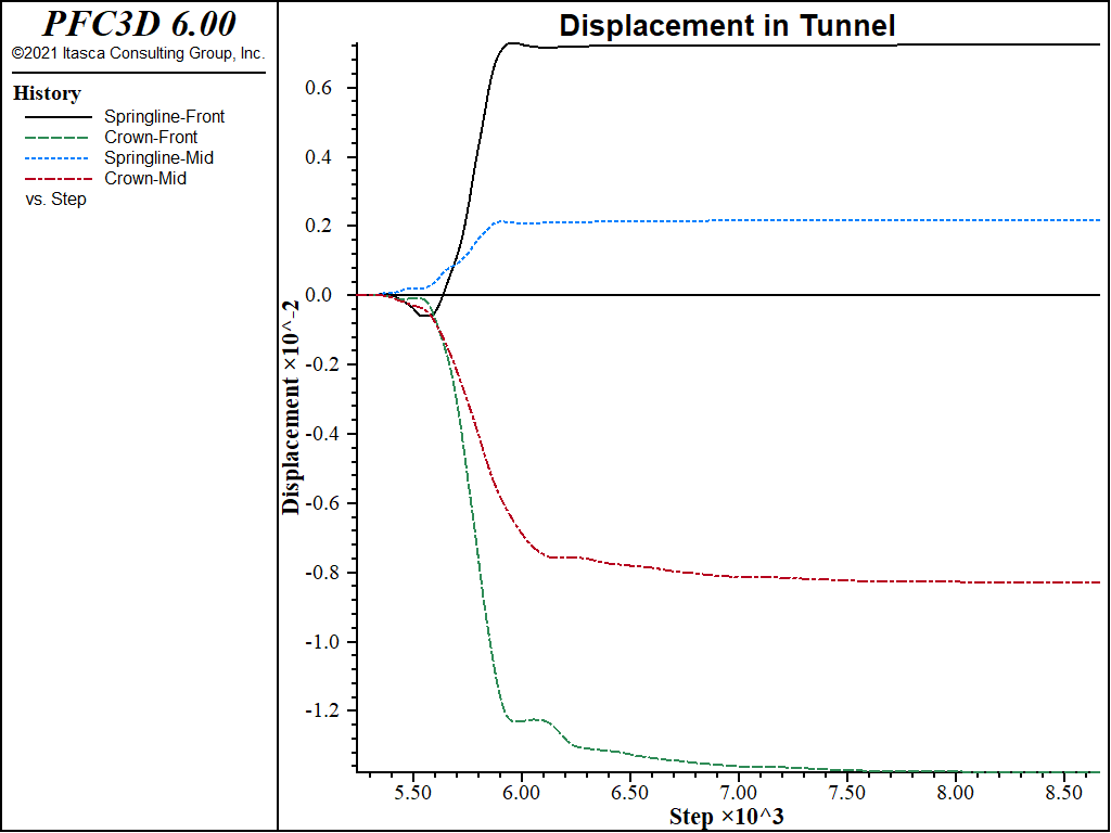
Again the displacements are initialized so we can see the effects of the excavation of the main tunnel. Significantly more displacement is measured in the service tunnel than was seen in the first two stages, and a greater asymmetry in the response. This is also evident in the contour plot of the displacement magnitude in the grid, and the minimum (i.e., major) principal stress (σ1) in the lining (see the second figure below).
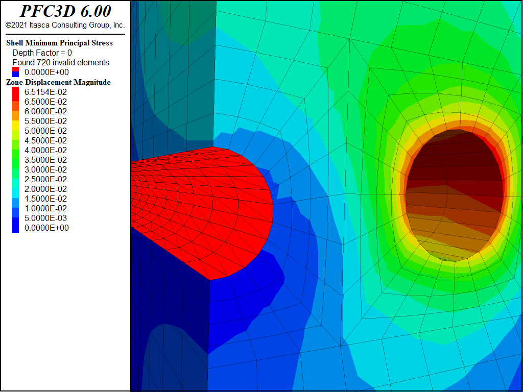
Figure 5: Contour plot of displacement magnitude in the grid and minimum principal stress in the lining after partial excavation of the main tunnel.
The modeling sequence may be repeated with different conditions of material properties, or locations of main tunnels relative to the service tunnel. If new tunnel locations are investigated, the grid must be regenerated and the model brought to an initial equilibrium state again. If different material properties are used, the model must be solved first for the response of the unlined service tunnel. Always remember that the model must be at an equilibrium state when the loading change is made.
Footnotes
| [1] | This approach is a simplistic simulation of the progressive advancement of the tunnel. For a more realistic model of sequential tunnel construction, see Excavation and Support for a Shallow Tunnel. |
| [2] | Of course, here we are referring to static mechanical processes. Transient calculations can be performed for groundwater flow and creep and thermal analyses with FLAC3D. Dynamic analysis can be performed with the dynamic option described in Dynamic Analysis. |
| Was this helpful? ... | PFC 6.0 © 2019, Itasca | Updated: Nov 19, 2021 |

