Free Vibration of a Cantilever Beam

Problem Statement

Note

To view this project in FLAC3D, use the menu command Help ‣ Examples…. Choose “Structure/Beam/FreeVibration” and select “FreeVibration.f3prj” to load. The main data file is shown at the end of this example. The remaining data files can be found in the project.

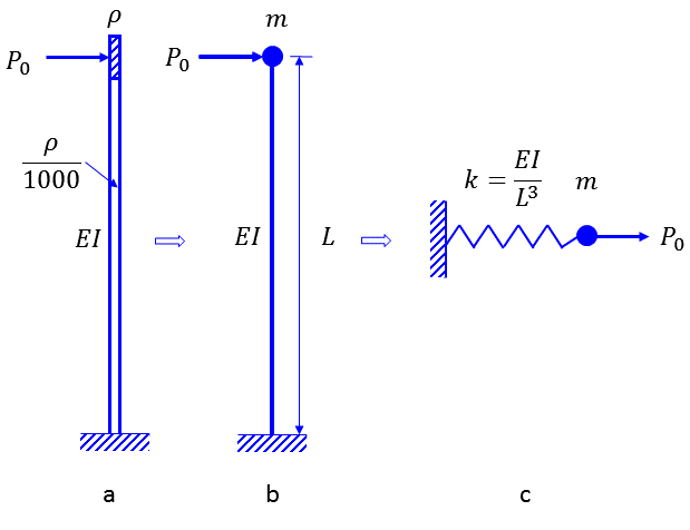
A cantilever beam is placed vertically (See Figure 1). At the beam top, the density is much bigger than elsewhere on the beam (Figure 1a). A horizontal force \(P_0 = k U_0\) is applied at the top mass centroid to ensure a static horizontal displacement of 0.001 at the beam top. The force is then released to let the beam vibrate. The model schematically shown in Figure 1a can be simplified into Figure 1b with a lumped mass \(m\) at the beam top. It can be further idealized as a single degree-of-freedom vibration system shown in Figure 1c, with a mass \(m\) and a stiffness \(k=EI/L^3\). The damping coefficient \(c\) will be assumed with various values. The FLAC3D model is based on Figure 1a using a beam element, and the FLAC3D solution will be compared with the analytical solution based on Figure 1c.

Figure 1: Free vibration of the cantilever beam.

The geometry and material parameters are summarized as follows.

Input Parameters:
\(E\)	2×1010
\(I\)	1
\(L\)	10
\(\rho\)	7.60×103
\(A\)	1
\(P_0\)	6×104
Derived Parameters:
\(m\)	1.52×104
\(k\)	6×107
\(U_0\)	0.001
\(T_n\)	0.1
\(\omega_n\)	20 \(\pi\)

The governing differential equation of free vibration for a single degree system with damping is

(1)\[m \ddot{u} + c \dot{u} + k u = 0\]

where \(u\) is the displacement, \(m\) is the mass, \(k\) is the stiffness, and \(c\) is the damping coefficient. The natural circular frequency is \(\omega_n = \sqrt{k/m}\), and the natural period is \(T_n = 2\pi/\omega_n\).

The critical damping coefficient is defined as \(c_{cr} = 2m\omega_n = 2\sqrt{km}\), and the damping ratio is defined as \(\zeta = c/c_{cr}\).

In this example, Rayleigh damping (\(c = \beta k + \alpha m\)) is assumed. For simplicity, only mass-proportional Rayleigh damping (\(\beta = 0\)) is considered here, so

(2)\[\zeta = {{\alpha m} \over {c_{cr}}} = {{\alpha} \over 2} \sqrt{m \over k} = {{\alpha} \over {2\omega_n}} = {{\alpha T_n} \over {4\pi}}\]

In this example, the initial condition at the dynamic stage is \(u(0) = U_0\) and \(\dot{u}(t)=0\). With these initial conditions, the analytical solution (Argris 1991) can be summarized as

1. No Damping   (\(\zeta=0\) or \(\alpha=0\)):

   (3)\[u(t) = U_0 \; \cos{(\omega_n t)}\]

2. Under Damping   (\(0 < \zeta < 1\) or \(0 < \alpha < 2\omega_n = 4\pi/T_n\)):

   (4)\[u(t) = U_0 \; e^{-\zeta \omega_n t} \left[ \cos{(\omega_D t)} + {\zeta \over {\sqrt{1-\zeta^2}}} \sin{(\omega_D t)} \right]\]

   where \(\omega_D = \omega_n \sqrt{1-\zeta^2}\).

3. Critical Damping   (\(\zeta = 1\) or \(\alpha = 2\omega_n = 4\pi/T_n\)):

   (5)\[u(t) = U_0 \; (1+\omega_n t) e^{-\omega_n t}\]

4. Over Damping   (\(\zeta > 1\) or \(\alpha > 2\omega_n = 4\pi/T_n\)):

   (6)\[u(t) = {U_0 \over 2\sqrt{(\zeta^2-1)}} \left[ c_2 e^{-c_1 \omega_n t} - c_1 e^{-c_2 \omega_n t} \right]\]

   where \(c_1 = \zeta-\sqrt{\zeta^2-1}\) and \(c_2 = \zeta+\sqrt{\zeta^2-1}\).

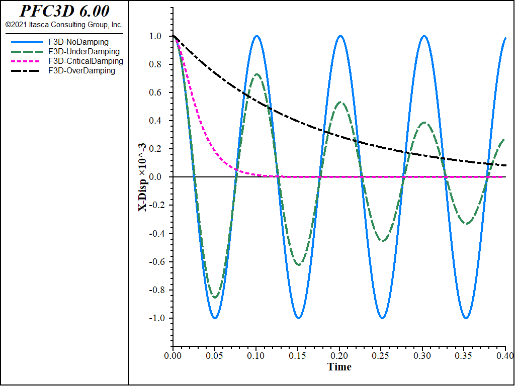
In the FLAC3D model, the beam is divided into 10 beam elements. A static horizontal force \(P_0\) is applied at the centroid of the lumped mass. After equilibrium is reached, the static displacement should be \(U_0 = P_0/k = 0.001\). The force is then released to let the cantilever beam freely vibrate at four different damping ratios, \(\zeta\) = 0%, 5%, 100%, and 500%, or \(\alpha\) = 0, \(2\pi\), \(40\pi\), and \(200\pi\) (since \(T_n\) = 0.1), to represent four cases, namely, no-, under-, critical-, and over-damping.

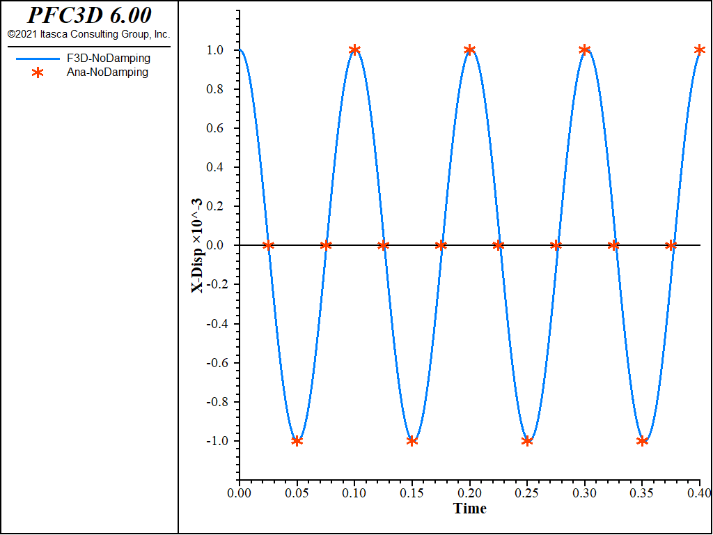
The FLAC3D solutions for all four cases are plotted in Figure 2. Comparisons with the analytical solutions are plotted in Figure 3 through Figure 6. In all cases a good fit is observed between the FLAC3D solution and the analytical solution.

Figure 2: FLAC3D solutions.

Figure 3: FLAC3D solution and analytical solution—no-damping (\(\alpha\) = 0 or \(\zeta\) = 0%).

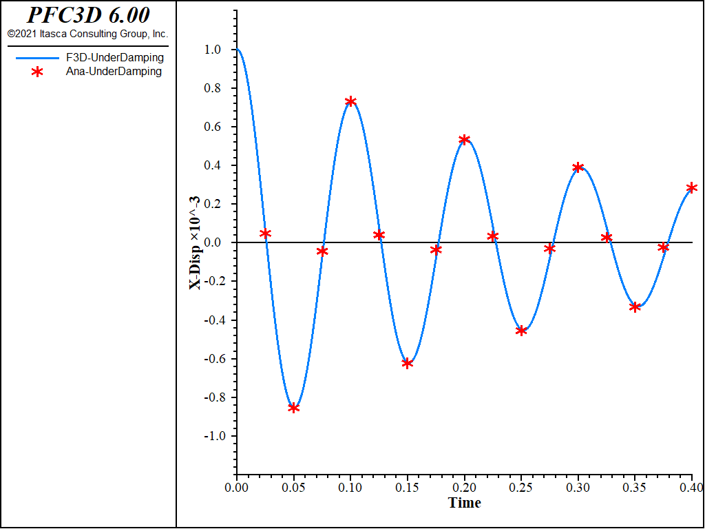
Figure 4: FLAC3D solution and analytical solution—under-damping (\(\alpha\) = 2 \(\pi\) or \(\zeta\) = 5%).

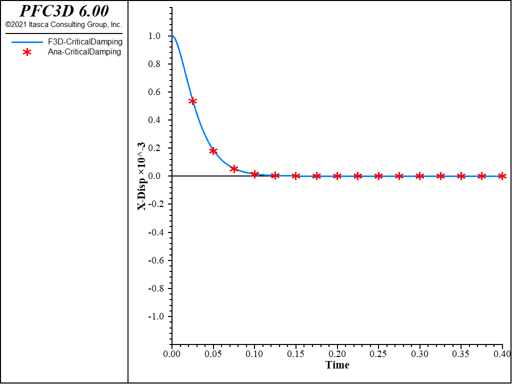
Figure 5: FLAC3D solution and analytical solution—critical-damping (\(\alpha\) = 40 \(\pi\) or \(\zeta\) = 100%).

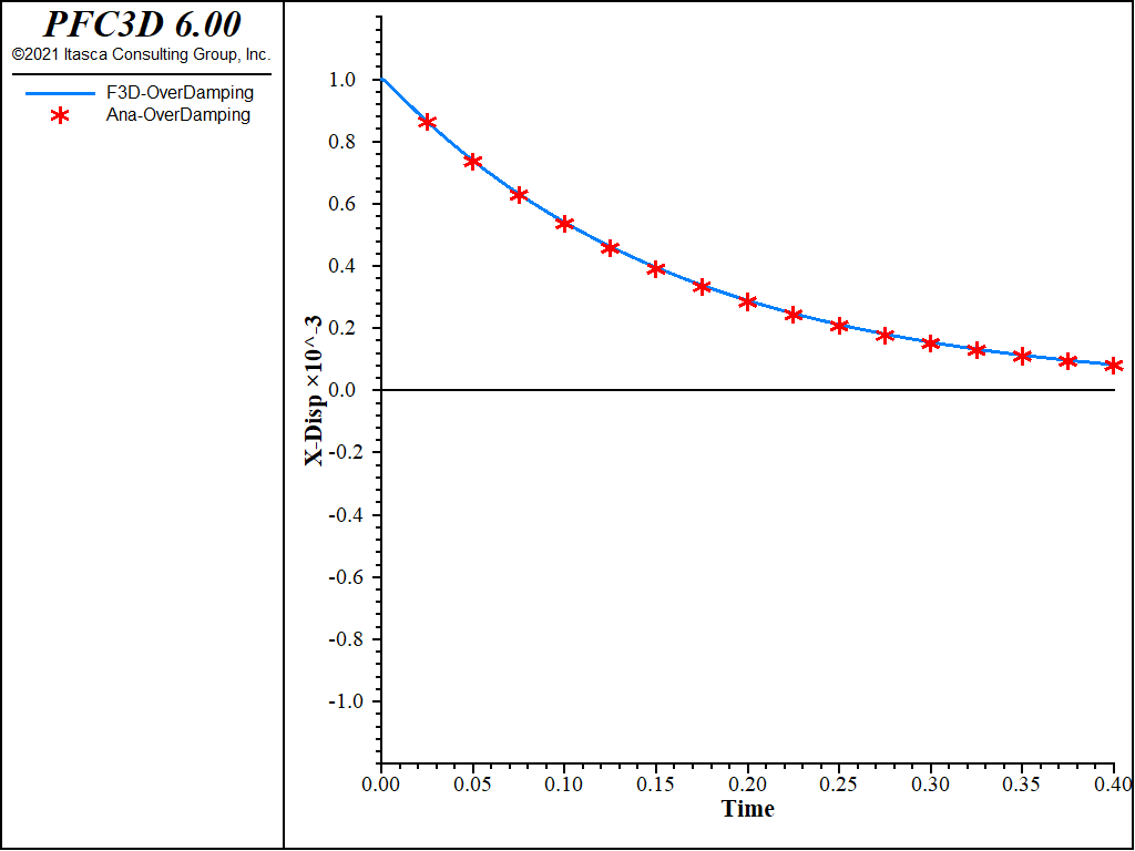
Figure 6: FLAC3D solution and analytical solution—over-damping (\(\alpha\) = 200 \(\pi\) or \(\zeta\) = 500%).

Reference

Argyris, J. & Mlejnek, H.-P. Dynamics of Structures. North-Holland, Amsterdam (1991).

Data File

FreeVibration.f3dat

model new
model largestrain off
model configure dynamic
model dynamic active off
;
call 'parameters'
@parameters
;
structure beam create by-line (0,0,0) (0,0,11) segments 11 id 1
structure beam property density [0.001*r] young @E poisson 0.3
structure beam property density @r range position-z 9.0 11.0
structure beam property cross-sectional-area @A moi-z @I moi-y @I moi-polar 0
structure node fix velocity range component-id 1
structure node fix rotation range component-id 1
structure node apply system global
structure node apply force [0.001*k] 0 0 range component-id 11
model solve ratio-local 1e-6
structure node apply remove force
model dynamic active on
model dynamic time-total 0
model dynamic timestep fix 1e-6
model history dynamic time-total
struct node history displacement-x component-id 11
struct node history velocity-x component-id 11
history interval 50
model save 'dynamic0'

;; No Damping
model solve time-total 0.4
history export 2 vs 1 table '1'
table '1' export 'NoDamping' truncate
model save 'NoDamping'

;;; Under Damping
model restore 'dynamic0'
[alpha = 0.05*c]
structure damping rayleigh 0 @alpha
model solve time-total 0.4
history export 2 vs 1 table '1'
table '1' export 'UnderDamping' truncate
model save 'UnderDamping'

;; Critical Damping
model restore 'dynamic0'
[alpha = c]
structure damping rayleigh 0 @alpha
model solve time-total 0.4
history export 2 vs 1 table '1'
table '1' export 'CriticalDamping' truncate
model save 'CriticalDamping'

;; Over Damping
model restore 'dynamic0'
[alpha = 5.0*c]
structure damping rayleigh 0 @alpha
model solve time-total 0.4
history export 2 vs 1 table '1'
table '1' export 'OverDamping' truncate
model save 'OverDamping'