FLAC3D Theory and Background • Fluid-Mechanical Interaction

Spreading of a Groundwater Mound

Note

To view this project in FLAC3D, use the menu command Help ? Examples…. Choose “Fluid/GroundwaterMound” and select “GroundwaterMound.f3dprj” to load. The project’s main data files are shown at the end of this example.

This problem studies the transient evolution of a groundwater mound within a porous medium. The mound spreads out and flows along an impervious base under the influence of gravity. It is assumed that the fluid is incompressible, and that the water is contained initially in a cylindrical region with radius \(r_{0}\) and height \(h_{0}\). The water saturation within the mound is equal to one, and Darcy’s law is applicable. The mound elevation is compared to an analytic solution as the elevation evolves with time.

Kochina et al. (1983) have derived the solution for the height, \(h\), of the mound. The solution, as given by Barenblatt (1987), assumes a hydrostatic pore-pressure distribution within the mound. In the case of zero residual saturation, it may be expressed in the form

(1)\[\hat{h}={{1}\over{8\sqrt{\hat{t}}}} \ [4-{{\hat{r}^{2}}\over{\sqrt{\hat{t}}}}]; \ \ \ \hat{r}\leq 2 \root 4 \of {\hat{t}}\]

where \(\hat{h} = h/h_{0}\), \(\hat{r} = r/r_{0}\), \(\hat{t} = t/t_{c}\), and the characteristic time is given as \(t_{c} = r_{0}^{2}/(2\kappa h_{0})\) with \(\kappa = k\rho _{w}g/(2n)\) (\(k\) is the mobility coefficient, \(\rho _{w}\) is water density, \(g\) is gravity and \(n\) is porosity).

This solution applies to long time scales, when the influence of the details of the initial mound geometry have disappeared.

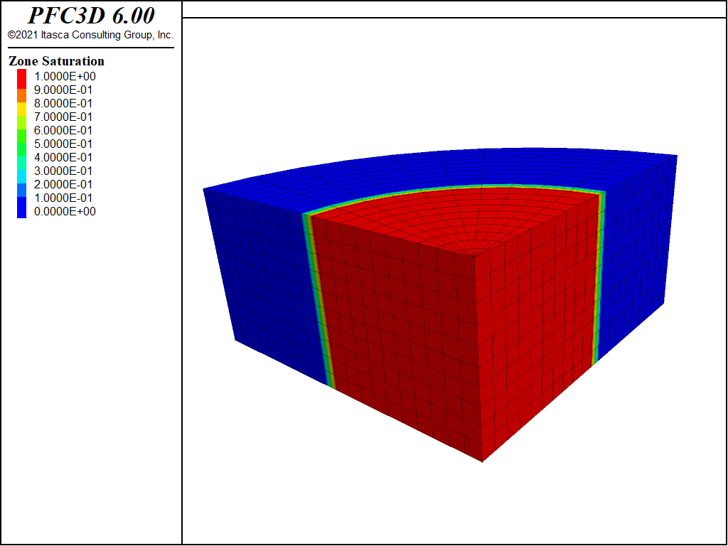
The results are presented in dimensionless form: the scaled geometrical parameters \(r_{0}\) = 1, \(h_{0}\) = 1 are used, and the scaled water properties \(k\) = 0.5 × 10^-4, \(\rho _{w}\) = 10³, and \(n\) = 0.5 are prescribed in the numerical simulation. To model incompressible flow, the bulk modulus of the fluid, \(K_{f}\), is given a value that is large compared to the pore-pressure variations in the simulation (\(K_{f}\) = 2 × 10⁵); the value \(g\) = 10 is used for gravity. The FLAC3D grid corresponds to a quarter cylinder and contains 2000 zones (see Figure 1). The radius of the model is 2, and its height is 1 unit. The initial saturation is 1 within the mound (radius = 1 unit, height = 1 unit), and zero outside. The initial pore-pressure distribution within the mound is hydrostatic. All boundaries are impermeable by default. As time goes on, the mound spreads out under its own weight. The simulation is conducted for a total dimensionless time value of \(\hat{t}\) = 0.85, with intermediate results at \(\hat{t}\) = 0.35, 0.45 and 0.65.

Figure 1: FLAC3D grid and initial state of saturated column.

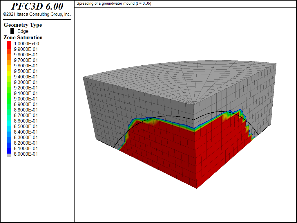
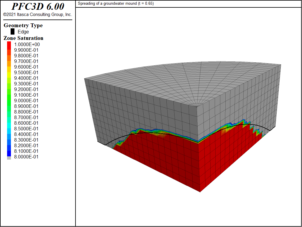
Saturation contours are sketched in Figure 2 to Figure 5. The analytic prediction for the mound height is calculated by a set of FISH functions and plotted for comparison in the figures (bold line).

Figure 2 corresponds to \(\hat{t}\) = 0.35; at that time, the initial shape of the mound still persists, and a comparison with the analytic solution is probably not yet appropriate. For larger times (see Figure 3 to Figure 5), the spreading of the groundwater mound described by Equation (1) is captured by the numerical solution with reasonable accuracy. The numerical estimate lags behind the analytical prediction; the discrepancy may be explained by the occurrence of residual saturation in the numerical solution and by the coarse discretization used in the simulation.

Figure 2: Saturation contours and analytical mound elevation at \(\hat{t}\) = 0.35.

Figure 3: Saturation contours and analytical mound elevation at \(\hat{t}\) = 0.45.

Figure 4: Saturation contours and analytical mound elevation at \(\hat{t}\) = 0.65.

Figure 5: Saturation contours and analytical mound elevation at \(\hat{t}\) = 0.85.

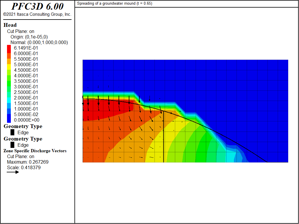
The sketch of flow vectors and head contours in Figure 6 corresponds to \(\hat{t}\) = 0.85. (The lack of smoothness in the contour plot is caused by the head jump across the phreatic surface.) Two regions with water flowing predominantly downward in the core of the mound and outward in its periphery can be seen in the figure. (The vertical bold line is drawn at the location where the time derivative of the analytical mound elevation vanishes: \(\partial \hat{h}/\partial t\) = 0.)

Figure 6: Head contours and analytical mound elevation at \(\hat{t}\) = 0.85

References

Barenblatt, G. Dimensional Analysis. Gordon and Breach Science Publishers (1987).

Kochina, I., N. Mikhailov and M. Filinov. “Groundwater Mound Damping,” Int. J. Engng. Sci., 21, 413-421 (1983).

Data File

GroundwaterMound.f3dat

model new
model largestrain off
fish automatic-create off
model configure fluid
; --- geometry ---
zone create cylinder size 20 10 10 point 1 (0 2 0) point 2 (0 0 1) point 3 (2 0 0
; --- fluid flow model ---
zone fluid cmodel assign isotropic
zone fluid property permeability 0.5e-4 porosity 0.5 biot 1
zone fluid biot on
zone gridpoint initialize biot 1e5
; if fluid modulus is specified:
; set fl biot off
; ini fmodulus 0.5e5
zone initialize fluid-density 1e3
zone gridpoint initialize fluid-tension 0
; --- initial conditions ---
model range create 'mound' cylinder end-1 0 0 -1 end-2 0 0 2 radius 1.01
zone gridpoint initialize saturation 0.0
zone gridpoint initialize saturation 1.0 range named-range 'mound'
zone gridpoint initialize pore-pressure 1e4 grad 0 0 -1e4 range named-range 'mound'
; --- settings ---
model gravity 0 0 -10
model mechanical active off
model fluid active on
model save 'mound0'
; --- test ---
model solve fluid time-total 0.35
model title "Spreading of a groundwater mound (t = 0.35)"
model save 'mound1'
model solve fluid time-total 0.45
model title "Spreading of a groundwater mound (t = 0.45)"
model save 'mound2'
model solve fluid time-total 0.65
model title "Spreading of a groundwater mound (t = 0.65)"
model save 'mound3'
model solve fluid time-total 0.85
model title "Spreading of a groundwater mound (t = 0.85)"
model save 'mound4'
return