Cable Structural Elements
Cable and bolt reinforcements in rock have two somewhat different functions. In hard rock subjected to low magnitude in-situ stress fields, failure is often localized and limited to wedges of rock directly adjacent to openings. The effect of the rock-bolt reinforcement here is to provide a local resistance to wedge displacement at the joint surfaces. In some cases, the bending, in addition to the axial stiffness of the reinforcement, may be important in resisting shear deformations. This type of bolt action may be modeled using pile structural elements, which have a flexural rigidity (see Pile Structural Elements). If bending effects are not important, cable structural elements are sufficient, because they provide a shearing resistance (by means of the grout properties) along their length. One can model reinforcing systems (e.g., cable bolts) in which the bonding agent (grout) may fail in shear over some length of the reinforcement. The numerical formulation that accounts for this shear behavior of the grout annulus is described in Shear Behavior of Grout Annulus.
Mechanical Behavior
Each cable structural element is defined by its geometric, material and grout properties. A cable element is assumed to be a straight segment of uniform cross-sectional and material properties lying between two nodal points. An arbitrarily curved structural cable can be modeled as a curvilinear structure composed of a collection of cable elements. The cable element behaves as an elastic, perfectly plastic material that can yield in tension and compression, but cannot resist a bending moment. A cable may be grouted such that force develops along its length in response to relative motion between the cable and the grid. The grout behaves as an elastic, perfectly plastic material, with its peak strength being confining stress dependent, and with no loss of strength after failure. Cable elements are suitable for modeling structural-support members in which tensile capacity is important, and for which axially directed frictional interaction with the rock or soil mass occurs.
Each cable element has its own local coordinate system, shown in Figure 1. This system is used to define the average axial cable direction. The cable element coordinate system is defined by the locations of its two nodal points, labeled as 1 and 2 in Figure 1. The element coordinate system is defined such that
- the centroidal axis coincides with the x-axis,
- the x-axis is directed from node-1 to node-2, and
- the y-axis is aligned with the projection of the global y- or x-direction (whichever is not parallel with the local x-axis) onto the cross-sectional plane.
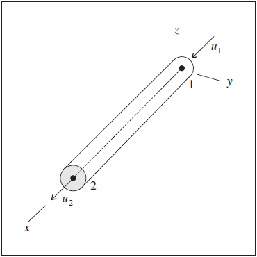
Figure 1: Cable element coordinate system and 2 active degrees-of-freedom of the cable finite element
The cable element coordinate system cannot be modified. It can be viewed with the Cable plot item and printed with the structure cable list system-local command. The nodal connectivity can be printed with the structure cable list information command.
The orientation of the node-local system for all nodes used by cable elements is set automatically at the start of a set of cycles (or when the model cycle 0 command is executed), such that the x-axis is aligned with the average axial direction of all cable elements using the node, and the yz-axes are arbitrarily oriented in the cable cross-sectional plane.
Cables support large-strain sliding (by setting the slide property to on) whereby the interpolation locations (used by the cable nodes to transfer forces and velocities to and from the zones — see Structural-Element Links) will migrate through the grid when running in large-strain mode. This allows one to calculate the large-strain, post-failure behavior of a cable whereby substantial sliding between the cable nodes and the zones occurs. If a cable node moves out of all zones, then a connection with the zones will not be reestablished if the node is later moved back into zones; however, the connection remains intact as the cable nodes slide between zones.
The two active degrees-of-freedom of the cable finite element are shown in Figure 1. For each axial displacement shown in the figure, there is a corresponding axial force. The stiffness matrix of the cable finite element includes only this single degree-of-freedom at each node to represent axial action within a cable structure.
The following four subsections describe (1) the axial behavior of the cable itself, (2) the shear behavior of the grout annulus, (3) the normal behavior at the grout interface, and (4) the means by which cables may be pretensioned. The behavior is described in terms of the cable properties listed in Properties (refer to this list for a summary of relevant notations).
Axial Behavior
The axial behavior of conventional reinforcement systems may be assumed to be governed entirely by the reinforcing member itself. The reinforcing member is usually composed of steel, and may be either a bar or a cable. Because the reinforcing member is slender, it offers little bending resistance (particularly in the case of a cable), and is treated as a one-dimensional structural member with the capacity to sustain uniaxial tension. (Compression is also allowed; however, when modeling support that is primarily loaded in compression, pile structural elements are recommended.)
A one-dimensional constitutive model is adequate for describing the axial behavior of the reinforcing member. The axial stiffness, K, is determined based on the reinforcement cross-sectional area, A, Young’s modulus, E, and element length, L, by the relation
A tensile- and compressive-yield strength, Ft and Fc, may be assigned to the cable element such that cable forces that are greater than these limits cannot develop (see Figure 2). If either Ft or Fc is not specified, the cable will have infinite strength for loading in that direction.
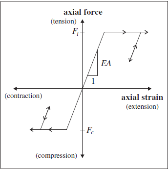
Figure 2: Cable material behavior for elements
Cables may break after sufficient accumulated plastic tensile strain. If the failure limit is set and the tensile strain goes over the value then the element is considered failed and will no longer sustain axial force in either compression or tension.
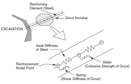
Figure 3: Mechanical representation of fully bonded reinforcement
Shear Behavior of Grout Annulus
The shear behavior of the cable-rock interface is cohesive and frictional in nature. The system is idealized (as shown in Figure 4 (a)), and represented numerically as a spring-slider system located at the nodal points along the cable axis (as shown in Figure 3). The shear behavior of the grout annulus during relative shear displacement between the cable/grout interface and the grout/rock interface (as shown in Figure 4 (b)) is described numerically by (1) the grout shear stiffness, kg, (2) the grout cohesive strength, cg, (3) the grout friction angle, ϕg, (4) the grout exposed perimeter, pg, and (5) the effective confining stress, σm ( Figure 4 (c)). The mechanical behavior of the grouted-cable system is depicted in terms of these parameters in Figure 5. Note that the grout properties associated with each cable element are averaged at cable nodes.
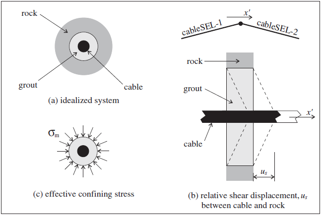
Figure 4: Idealization of grouted-cable system
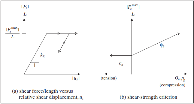
Figure 5: Grout material behavior for cable elements
The effective confining stress, σm, acts in the plane perpendicular to the cable axis, and is computed at each nodal point along the cable axis, based on the stress acting in the zone to which the nodal point is linked. Denote the cable-axis direction as x′, and denote the principal stresses acting in the y′z′-plane as σ1 and σ2, such that σ1>σ2 (tension positive). Then the value of σm is taken as
where: p = pore pressure
In computing the relative displacement at the cable-rock interface, an interpolation scheme is used to calculate the displacement of the rock in the cable axial direction at each cable node, based on the displacement field in the zone to which the node is linked. The interpolation scheme uses weighting factors that are determined by the distance to each of the gridpoints of the zone. The same interpolation scheme is used to apply forces developed at the cable-rock interface back to the gridpoints of the zone.
Normal Behavior at Grout Interface
As explained above, an interpolated estimate of grid velocity is made at each cable node. The velocity normal to the cable-axis direction is transferred directly to the node (i.e., the cable node is “slaved” to the grid motion in the normal direction). The node exerts no normal force on the grid if the two cable elements that share the node are colinear; however, if the two elements are not colinear, then a proportion of their axial forces will act in the normal direction. This net force acts both on the grid and on the cable node (in opposite directions). Thus, an initially straight cable can sustain normal loading if it is allowed finite deflection, using the large-strain solution mode.
Pretensioning
Cables may be pretensioned via the structure cable apply tension command. A positive value assigns a tensile axial force into all of the cable elements that fall within the range. This tension will be maintained until released with the structure cable apply tension active off command. Note that removing the tension apply condition does not change the current axial force in the cable element, it just removes the condition maintaining that force at a specific level.
In practice, pretensioned cables may be fully grouted, or they may be left ungrouted over part of their length. In either case, some anchorage length is provided (usually at the far end) to support the cable during pretensioning. To simulate this pretensioning, one need only specify anchorage properties for the cable elements making up the anchorage length, and other properties (e.g., cg=0) for the elements making up the free length.
It is important to note that the cable with specified pretension is initially unlikely to be in equilibrium with other structural elements or the model grid to which it is linked. In other words, some displacement of the cable nodes and linked entities is probably required to achieve equilibrium. As a result, properly pretentioning cables generally is done in three commands:
struct cable apply tension value 1000 range group 'pretension'
model solve
struct cable apply tension active off
The first command applies tension to a specific set of cable elements (previously tagged with the pretension group name for this purpose). The second command solves to equilibrium. The third command removes the applied tension value, so that the cable will respond naturally from then on.
For an example of this in practice, please see Installation of a Triple-Anchored Excavation Wall or Impermeable Concrete Caisson Wall with Pretensioned Tiebacks.
Response Quantities
Cable responses include force, stress and yield state of the cable element itself, and stress, displacement and slip state of the shear coupling springs that represent the grout. Additional coupling-spring information includes the current loading direction and the confining stress. The cable responses can be accessed via FISH and
- printed with one of the keywords available to the the
structure cable listcommand, - monitored with the
structure cable historycommand, and - plotted with the Cable plot item.
The sign of the grout stress refers to the average axial cable direction such that positive grout stresses act on the cable in the positive average axial cable direction. This sign convention assumes that the set of elements making up the cable are oriented consistently, such that their local coordinate systems form a continuous description of the cable orientation. Such will be the case if the cable is created using the structure cable create command. The nodes of each element so created will be ordered such that the overall cable direction goes from the first point to the second point. The nodal connectivity can be printed with the structure cable list information command.
Properties
Each cable element possesses 12 properties:
- density, mass density, ρ (optional — needed if dynamic mode or gravity is active) [M/L3]
- young, Young’s modulus, E [F/L2]
- grout-cohesion, grout cohesive strength (force) per unit length, cg [F/L]
- grout-friction, grout friction angle, ϕg [degrees]
- grout-stiffness, grout stiffness per unit length, kg [F/L2]
- grout_perimeter, grout exposed perimeter, pg [L]
- slide, large-strain sliding flag (default: off)
- slide-tolerance, large-strain sliding tolerance
- thermal-expansion, thermal-expansion coefficient, αt [1/T] (optional — used for thermal analysis)
- cross-section-area, cross-sectional area, A [L2]
- yield-compression, compressive yield strength (force), Fc [F]
- yield-tension, tensile yield strength (force), Ft [F]
The area, modulus and yield strength of the cable are usually readily available from handbooks, manufacturer’s specifications, etc. The grout properties are more difficult to estimate. The grout annulus is assumed to behave as an elastic-perfectly plastic solid. As a result of relative shear displacement, ut, between the tendon surface and the borehole surface, the shear force, Ft, mobilized per length of cable is related to the grout stiffness, kg:
Usually, kg can be measured directly in laboratory pull-out tests. Alternatively, the stiffness can be calculated from a numerical estimate for the elastic shear stress, τG, obtained from an equation describing the shear stress at the grout/rock interface (St. John and Van Dillen 1983):
| where: | Δu | = | relative displacement between the element and the surrounding material; |
| G | = | grout shear modulus; | |
| D | = | reinforcing diameter; and | |
| t | = | annulus thickness. |
Consequently, the grout shear stiffness, kg, is simply given by
In many cases, the following expression has been found to provide a reasonable estimate of kg for use in the program:
The one-tenth factor helps to account for the relative shear displacement that occurs between the host-zone gridpoints and the borehole surface. This relative shear displacement is not accounted for in the present formulation.
The maximum shear force per cable length in the grout is determined by the relation illustrated in Figure 2. The values for bond cohesive strength, cg, and friction angle, ϕg, can be estimated from the results of pull-out tests conducted at different confining pressures or, should such results not be available, the maximum force per length may be approximated from the peak shear strength (St. John and Van Dillen 1983):
where τI is approximately one-half of the uniaxial compressive strength of the weaker of the rock and grout, and QB is the quality of the bond between the grout and rock (QB = 1 for perfect bonding).
Neglecting frictional confinement effects, cg may then be obtained from
Failure of reinforcing systems does not always occur at the grout/rock interface. Failure may occur at the reinforcing/grout interface, as is often true for cable reinforcing. In such cases, the shear stress should be evaluated at this interface. This means that the expression (D+2t) is replaced by (D) in (2).
The calculation of cable element properties is demonstrated by the following example. A 25.4 mm (1 inch)-diameter locked-coil cable was installed at 2.5 m spacing. The reinforcing system is characterized by several properties:
| cable diameter (D) | 25.4 mm |
| hole diameter (D+2t) | 38 mm |
| cable modulus (E) | 98.6 GPa |
| cable ultimate tensile capacity | 0.548 MN |
| grout compressive strength | 20 MPa |
| grout shear modulus (Gg) | 9 GPa |
| friction (ignored) | 0 |
Two independent methods are used in evaluating the maximum shear force in the grout. In the first method, the bond shear strength is assumed to be one-half the uniaxial compressive strength of the grout. If the grout-material compressive strength is 20 MPa, and the grout is weaker than the surrounding rock, the grout shear strength is then 10 MPa.
In the second method, reported pull-out data are used to estimate the grout shear strength. The report presents results for 15.9 mm (5/8 inch)-diameter steel cables grouted with a 0.15 m (5.9 inch) bond length in holes of varying depths. The testing indicated capacities of roughly 70 kN. If a surface area of 0.0075 m2 (0.15 m × 0.05 m) is assumed for the cables, then the calculated maximum shear strength of the grout is
This value agrees closely with the 10 MPa estimated above, and either value could be used. Assuming failure occurs at the cable/grout interface, the maximum bond force per length is (using (2) with D+2t replaced by D)
The grout stiffness, kg, is estimated from (1). For the assumed values shown above, a grout stiffness of 1.5 × 10¹⁰ N/mm is calculated.
Another example estimation of grout properties from pull-out tests is presented in Simulation of Pull-Tests for Fully Bonded Rock Reinforcement
Example Applications
Simple examples are given to illustrate the use of cables.
A complete list of examples that use cable elements is available in Structural Cable Examples.
Commands & FISH
| Was this helpful? ... | FLAC3D © 2019, Itasca | Updated: Feb 25, 2024 |