Tunnel Excavation in a Bonded Block Model

Problem Statement

Note

The project file for this example may be viewed/run in 3DEC.[1] The data files used are shown at the end of this example.

A 10x5 m rectangular tunnel is excavated in fractured crystalline rock at a depth of 1100 m. The area of interest is represented by tetrahedral blocks bonded together, and the rest of the model is elastic continuum. Fragmentation is examined in the area of interest. The example also shows the effects of suppressing the vertex-vertex contacts.

Calibration

A bonded block model (BBM) is composed of many blocks bonded together. The blocks are usually tetrahedra. The properties of the intact rock are usually known from lab studies and these properties are assigned to the zones that make up the blocks. The rock mass properties may be determined from GSI or some other rock classification scheme used to estimate the effect of fractures on the rock strength and stiffness. To create a model of the rock mass, the user needs to specify the joint properties that yield the desired rock mass behavior. This is an inverse problem that usually involves guessing at some properties and then running a test and adjusting the properties until the desired behavior is observed.

Because bonded block models are computationally expensive, usually only a small volume of the entire model is represented this way. The rest of the model is represented by an equivalent continuum. The stiffness of the equivalent continuum should be the same as the macro stiffness of the BBM. The macro stiffness of the BBM is obtained by performing a compression test on a BBM sample. It is important that the block sizes in the calibration test are the same as the blocks that will be used in the field scale model since the joint spacing affects the stiffness.

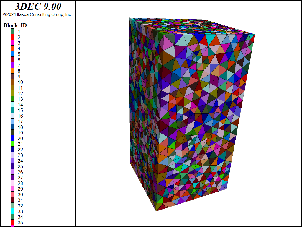
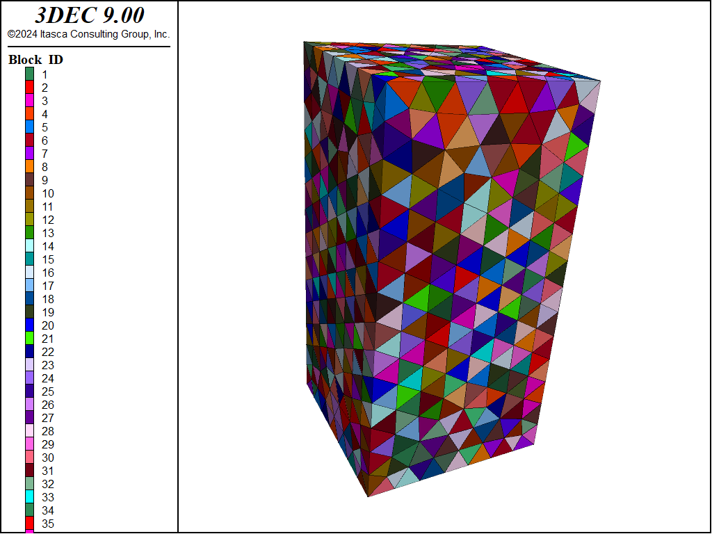
The elastic properties of the BBM in this model are shown in Table 1. To determine the macro stiffness of the material, a 10x10x20 m sample is created and subjected to an unconfined compression test. The model is created by filling a box with tetrahedral elements (block generate from-geometry). Figure 1 shows the model. The random keyword is used to give some randomness to the block sizes (they will be assigned a uniform size distribution between the minimum and maximum specified edge lengths). This is useful to prevent a very regular packing which may occur when all zones are the same size (Figure 2).

In this example, the formation of vertex-vertex contacts is suppressed using the command block contact vertex-vertex off. This reduces memory and and run time without having a significant effect on the results (this is discussed further below).

Table 1: Model Elastic Properties

Property	Value
Intact Young’s Modulus (GPa)	60
Intact Poisson’s Ratio	0.25
Contact normal stiffness (GPa/m)	1050
Contact shear stiffness (GPa/m)	525

Figure 1: 3DEC calibration model showing blocks generated with the random keyword.

Figure 2: 3DEC calibration model showing blocks generated without the random keyword.

The UCS test is run by applying velocities to the top and bottom gridpoints and monitoring the vertical stress (sum of reaction forces on the top and bottom gridpoints divided by the cross-sectional area), and the vertical and lateral strains (displacement differences between selected gridpoints on the edges of the model). The data file for this model is shown below (bbm_calibration.dat).

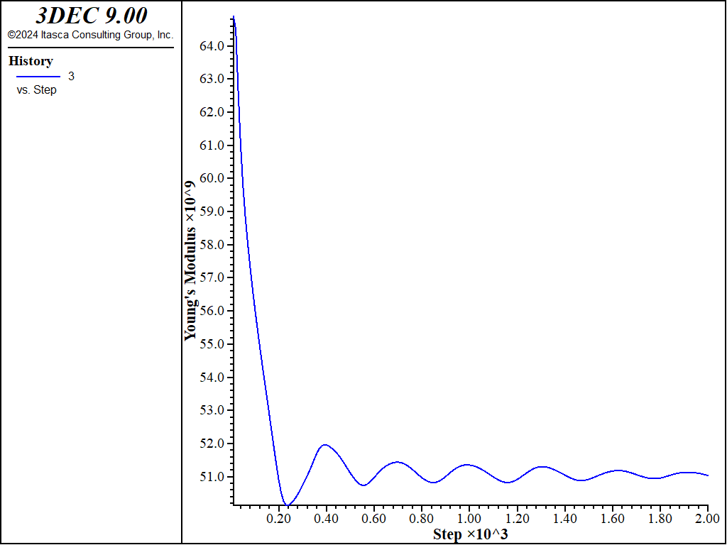
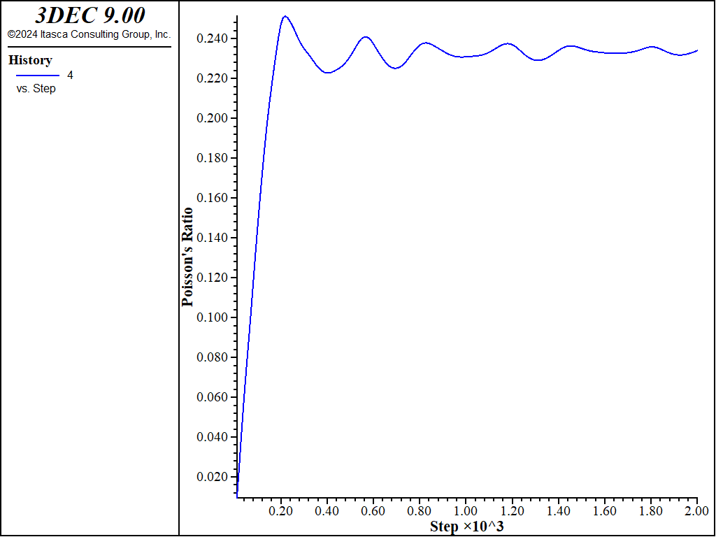
Young’s Modulus is then calculated from vertical stress / vertical strain and Poisson’s Ratio is calculated from horizontal strain / vertical strain. The evolution of Young’s modulus and Poisson’s Ratio in the model are shown in Figure 3 and Figure 4. From these graphs it can be seen that the macro Young’s modulus is approximately 51 GPa and the macro Poisson’s Ratio is approximately 0.23. These values will be used in the equivalent continuum portion of the tunnel model.

Figure 3: Evolution of Young’s Modulus in the calibration model.

Figure 4: Evolution of Poisson’s Ratio in the calibration model.

Tunnel Model

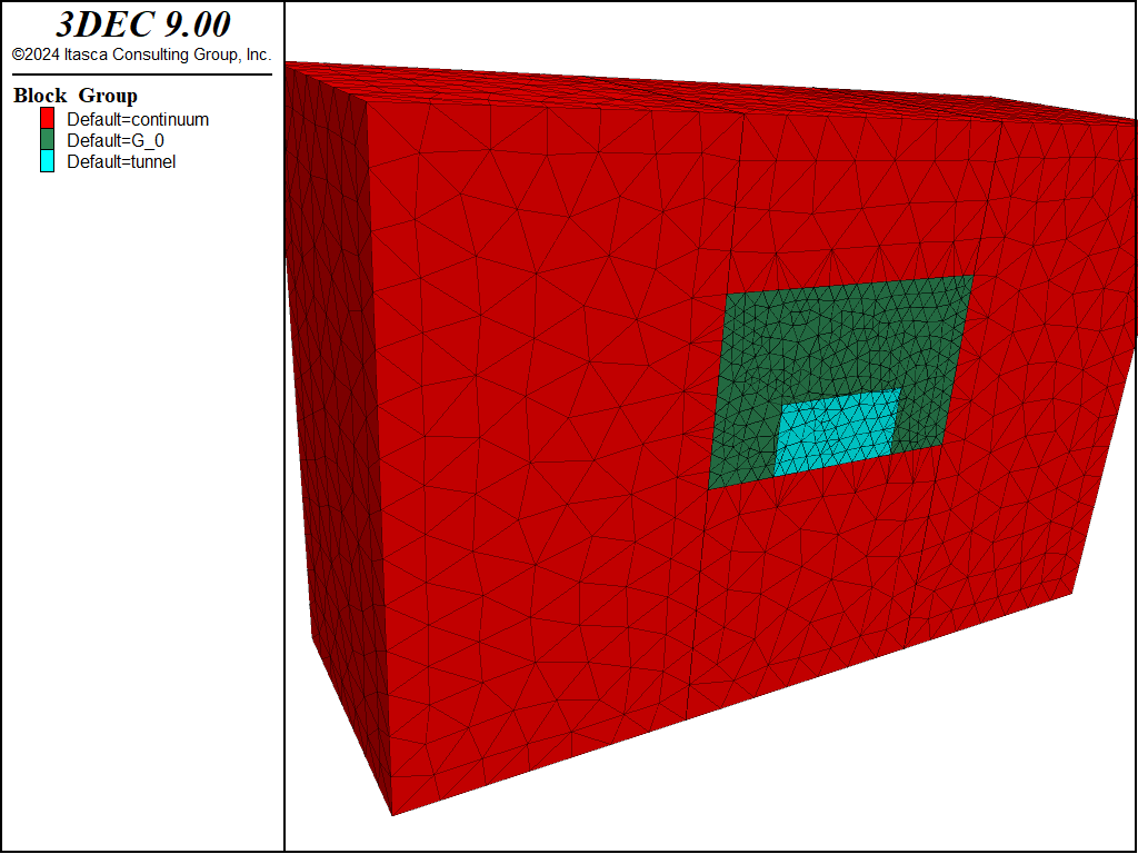
For this example, it is assumed that the area of interest is above the tunnel. The model is created by first making a 60x20x40 m block. The region of interest above the proposed tunnel is then cut out with block cut joint-set commands. The cut out block is then deleted and the volume is filled with tetrahedral elements as in the above calibration example. The tunnel is then cut out and the blocks inside of the tunnel are grouped. Finally, the model is zoned with coarser zones in the continuum region. Figure 5 shows the model.

As in the calibration model, the formation of vertex-vertex contacts is suppressed using the command block contact vertex-vertex off. This reduces memory and and run time without having a significant effect on the results.

Figure 5: 3DEC tunnel model.

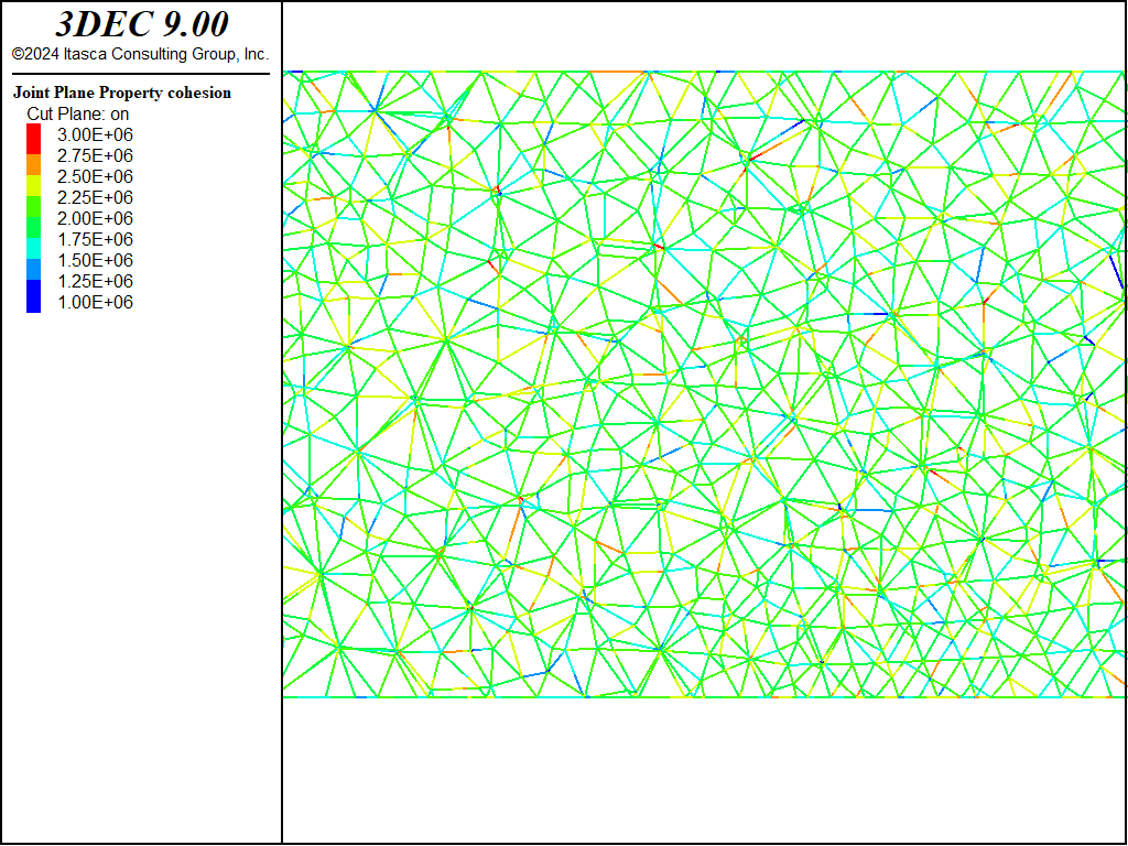
Table 2 summarizes the contact strength parameters. The contacts are assigned the Mohr-Coulomb joint constitutive model. The joint strength properties are assigned a Gaussian distribution. A cross-section showing joint cohesion values is shown in Figure 6

Table 2: Contact Strength Properties

Property	Mean Value	Standard Deviation
Contact dilation (degrees)	5
Contact friction (degrees)	45	5
Contact cohesion (MPa)	2	0.5
Contact tension (MPa)	0.9	0.2

Figure 6: Cross-section of the model showing joint cohesion values.

The in-situ stress is lithostatic, with the vertical stress equal to the weight of the overburden material and the horizontal stresses equal to twice the vertical.

All boundaries are fixed except the top, on which a vertical stress is applied. Gravity is turned on and the model is solved in large strain.

Tunnel Excavation

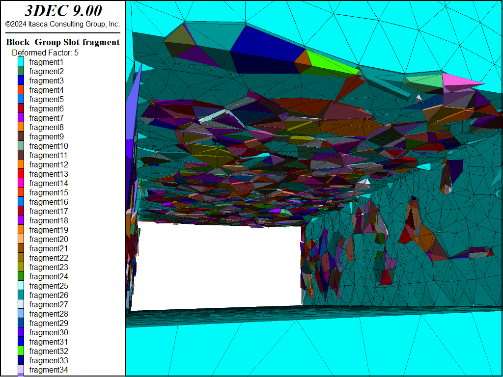
Gradual excavation is simulated using the block relax command. After the relaxation, the model is run for another 5000 steps. The model solve command cannot be used here because blocks are falling from the roof and the model never comes to equilibrium.

After 5000 steps, fragments are computed as shown in Figure 7.

Figure 7: Fragments in the model at the end of the simulation.

Vertex-Vertex Contacts

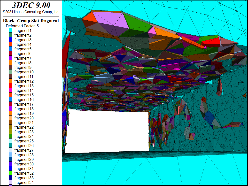
The same model was run with vertex-vertex contacts on. This results in approximately 800,000 vertex-vertex contacts. The resulting fragments for this model are shown in Figure 8. Some slight differences can be seen, but the overall behavior is similar. This model uses 10% more memory and takes 20% longer to run.

Figure 8: Fragments in the model at the end of the simulation for a model with vertex-vertex contacts.

Data Files

bbm_calibration.dat

model new
model random 10000

geometry set 'box'
geometry generate box -5 5 -5 5 -10 10

; suppress formation of vertex-vertex contacts
block contact vertex-vertex off

; generate tet blocks with randomness
block generate from-geometry set 'box' minimum-edge 0.6 maximum-edge 1.4 random

block zone generate edgelength 1.4

; assign properties
block zone cmodel assign elastic
block zone property density 2750 young 60e9 poiss 0.25

block contact jmodel assign elastic
block contact property stiffness-normal 1050e9 stiffness-shear 525e9 

; gps on the boundary
block gridpoint group 'top' range position-z 10
block gridpoint group 'bottom' range position-z -10

; set up for histories
fish define setup
  global top_gps = block.gp.list(block.gp.isgroup(::block.gp.list,'top'))
  global bottom_gps = block.gp.list(block.gp.isgroup(::block.gp.list,'bottom'))
  
  global area = 10*10  
  global height = 20
  global width = 10 
  global depth = 10
  global gp_left = block.gp.near(-5,0,0)
  global gp_right = block.gp.near(5,0,0)
  global gp_front = block.gp.near(0,-5,0)
  global gp_back = block.gp.near(0,5,0)
  global gp_top = block.gp.near(0,0,10)
  global gp_bottom = block.gp.near(0,0,-10)
end
[setup]

; stress/strain histories
fish define szz
  ; compression positive
  local szz_local = -list.sum(block.gp.force.reaction.z(::top_gps))
  szz_local += list.sum(block.gp.force.reaction.z(::bottom_gps))
  szz_local /= (area*2.0)
  global ezz = (block.gp.disp.z(gp_bottom) - block.gp.disp.z(gp_top))/height
  global young = szz_local / ezz

  local lat_strain1=(block.gp.disp.x(gp_right)-block.gp.disp.x(gp_left))/width
  local lat_strain2=(block.gp.disp.y(gp_back)-block.gp.disp.y(gp_front))/depth
  global poiss = 0.5*(lat_strain1+lat_strain2) / ezz
  szz = szz_local
end

fish history szz
fish history ezz
fish history young
fish history poiss

; set up initial velocities to speed analysis
block gridpoint initialize velocity-z 0 gradient 0 0 -0.005

block gridpoint apply velocity-z 0.05 range group 'bottom'
block gridpoint apply velocity-z -0.05 range group 'top'

model large-strain off

model cycle 2000

model save 'calibration'

bbm_tunnel.dat

model new
model random 10000

; thistory prevents unjoining of blocks when new cuts are made
block join-by-contact on

block create brick -30 30 -10 10 -20 20

; cut out bbm region
block cut joint-set dip 90 dip-direction 90 origin -10 0 0 
block cut joint-set dip 90 dip-direction 90 origin 10 0 0 
block cut joint-set origin 0 0 10 range position-x -10 10
block cut joint-set origin 0 0 -2.5 range position-x -10 10
block join
block group 'continuum'

; delete bbm block and make bbm
block delete range position-x -10 10 position-z -2.5 10

geometry set 'box'
geometry generate box -10 10 -10 10 -2.5 10

; suppress formation of vertex-vertex contacts
block contact vertex-vertex off

; generate tet blocks with randomness
block generate from-geometry set 'box' minimum-edge 0.6 maximum-edge 1.4 random

; cut out tunnel
block cut joint-set origin 0 0 2.5 jointset-id 99 range position-x -5 5 
block cut joint-set dip 90 dip-direction 90 jointset-id 99 origin -5 0 0 ...
  range position-z -2.5 2.5
block cut joint-set dip 90 dip-direction 90 jointset-id 99 origin 5 0 0 ...
  range position-z -2.5 2.5
block group 'tunnel' range position-x -5 5 position-z -2.5 2.5

; zone
block zone generate edgelength 2.8 range group 'continuum'
block zone generate edgelength 1.4

; assign bbm zone properties
block zone cmodel assign elastic
block zone property density 2750 young 60e9 poiss 0.25

; assign equivalent continuum zone properties
block zone property density 2750 young 51e9 poiss 0.23 range group 'continuum'

; assign contact properties
block contact jmodel assign mohr
block contact property stiffness-normal 1050e9 stiffness-shear 525e9 dilation 5
block contact prop-dist friction 45 deviation-gaussian 5
block contact prop-dist cohesion 2e6 deviation-gaussian 0.5e6
block contact prop-dist tension 9e5 deviation-gaussian 0.2e5 

block contact material-table default property stiffness-normal 1050e9 ...
  stiffness-shear 525e9 friction 45 dilation 5

; make construction joints elastic
block contact jmodel assign elastic range joint-set 99
block contact property stiffness-normal 1050e9 stiffness-shear 525e9 ...
  range joint-set 99

; initial conditions
; assume 1100 m below the surface and horizontal = 2*vertical
model gravity 9.81

[overburden = -9.81*2750*1100]
block insitu topography ratio-x 2 ratio-y 2 overburden [overburden]

; boundary conditions
block face apply stress-zz [overburden] range position-z 20
block gridpoint apply velocity-y 0. range position-y -10
block gridpoint apply velocity-y 0. range position-y 10
block gridpoint apply velocity-x 0. range position-x -30
block gridpoint apply velocity-x 0. range position-x 30
block gridpoint apply velocity 0 0 0 range position-z -20

; histories
block history name 'top-middle' displacement-z position 0 0 2.5

model large-strain on

model solve

model save 'tunnel-initial'

Endnotes

[1]

To view this project in 3DEC, use the program menu.

Help ▼ Examples…

  ⮡   3DEC
   ⮡   ExampleApplicatoins
    ⮡   BBM_Tunnel
     ⮡   BBM_tunnel.prj