Rigid Block Model of Tunnel Excavation
Problem Statement
Note
The project file for this example may be viewed/run in PFC.[1] The data files used are shown at the end of this example.
This example simulates the sequential excavation of a tunnel in a fractured rock mass. Stresses are installed in the initial, zero-porosity Bonded Block Model (BBM) consistent with a tunnel at 400 m depth, where the lateral stresses are larger than the overburden stress. The tunnel, excavation boundaries and fractures are cut into the graded tetrahedral model. The subspringnetwork contact model provides both the elastic and failure response of the rock mass. This is an implementation of the Rigid Body Spring Network (RBSN) approach with subcontacts. The Mohr Model model is used to model the behavior of the fracture surfaces. As excavation continues, damage accrues around the previously excavated sections. In addition, slip occurs on fractures outside of the damage region.
Geometry Creation
The rblock construct command is used to create rigid blocks inside a parallelepiped domain. The resulting tetrahedra form a zero-porosity representation of the rock mass, with specified maximum edge length, that conforms to the boundary of the parallelepiped. Geometry node extra variables are used to insert randomness into the resulting rigid blocks and to also grade the rigid block sizes as a function of distance from the center of the tunnel. Subsequent to model creation, the boundaries are identified for future reference, prior to block scaling to ensure initial overlap.
The tunnel geometry is imported from a dxf file and cut into the rigid blocks. A group is assigned to the cut facets to assist in support force installation, and the blocks inside the tunnel are also grouped. To allow for clean 2 m long progression, the tunnel blocks are cut by a joint set with 2 m spacing. Finally a set of fractures are created and cut into the blocks to simulate a background fracture pattern. In all cases slivers are not removed when cutting. Finally groups are assigned to block facets for easy support force application.
For a zero-porosity model such as this one, one would expect that the contacts responsible for the elastic response would be located between the faces of adjacent tetrahedra, not located between tetrahedra edges or vertices. For non-bonded contacts, the contact location is defined as the centroid of the volume of overlap. Thus, in order for the face-face contacts to be identified and the contact locations to lie at the centroids of the face-face overlap regions, the rigid blocks are scaled (see the rblock dilate command). Should the model be bonded in this state, there would be many edge-edge and vertex-vertex contacts that do not contribute to the elastic response and greatly slow the computation. To effectively remove these contacts during the simulation, a criteria involving the facet areas is used wherein a contact is not created unless its area is greater than some fraction of the total surface area of the rigid block. This approach is preferred to the previous examples using erosion, especially for small strain simulations.
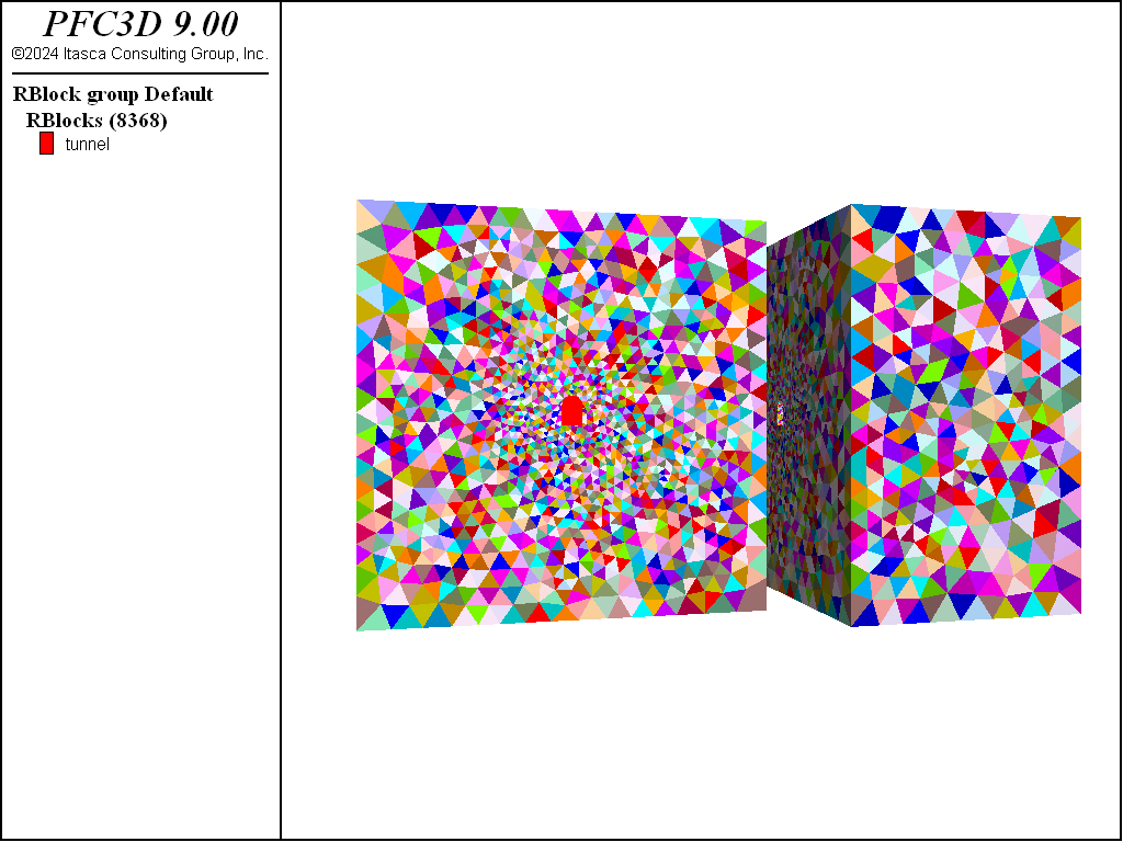
Figure 1: Initial configuration of the rigid blocks after cutting and scaling.
Stress Initialization
Prior to contact creation the rblock contact-resolution command is given to ensure that the actual overlap area is used, that edge-edge and vertex-vertex contacts are remediated, and that stress is accumulated in the rigid blocks. This last step is required for the springnetwork or subspringnetwork models to provide an effective Poisson correction. Contacts are created and contact detection is turned off as the model will be run in small strain. The contact tensile strengths are assigned from a Weibull distribution and the cohesive strengths are fixed relative to the tensile strengths. Contacts are identified that are associated with background fractures and the mohr model is assigned with fixed stiffnesses per unit area. It is important to note that the area method should be used with the mohr model when rigid blocks are involved so that the area is fixed.
The RBSN approach has been primarily used in the literature to model conformal Voronoi meshes. Tetrahedral based models have some advantages including ease of creation, lower coordination number (i.e., fewer contacts per rigid block) and greatly diminished interlocking between adjacent blocks. This example additionally uses cutting which can result in very small, poor aspect-ratio rigid blocks. For quasi-static simulations these slivers shouldn’t impact the bulk material response appreciably. In some cases, instabilities can occur due to the Poisson correction when poor aspect-ratio slivers are involved. The subspringnetwork model can automatically check for instabilities based on a convergence criteria, providing a practical way of retaining slivers in quasi-static analyses without impacting the material response. This will not work well for dynamic simulations, though, as the timestep would suffer severely with such small slivers. Finally the out-of-plane velocities and spins are fixed at the boundaries and the model is first solved elastically (i.e., without contact failure or slip). The model is subsequently solved to equilibrium allowing for contact failure and/or slip.

Figure 2: Minimum and maximum principal stresses after equilibration.
Tunnel Excavation
After the preceding steps the environment is enhanced to track cracks in the bulk material and to apply support stresses. The former is accomplished by catching the \(bond_broken\) event for the subpringnetwork model. The \(bond_break\) event triggers when a subcontact is broken, whereas the \(broken\) event triggers when all three subcontacts are broken. Fractures are created for each contact when it is completely broken in different DFNs so that one can visualize the progression of failure. The support stresses are applied with the rblock facet apply command. At each cycle the out-of-balance force and moment are applied to the identified rigid blocks. A simple FISH function is called for each rigid block to compute a multiplicative factor that is applied to the out-of-balance forces/moments. The multiplicative factor is 1 for a fixed number of cycles and then linearly ramps to 0 over a fixed number of cycles for all rigid blocks with the apply condition. In addition, the magnitude of the out-of-balance force on the support blocks divided by the area of the tunnel surface, or the average applied stress, is cataloged.
For each of the four excavation stages a unique DFN is created, the tunnel blocks are deleted for that stage, the support blocks are identified for that stage, the \(rblist\) FISH list used to compute the \(appliedStress\) is updated, the tunnel surface area is updated, the old apply conditions are removed (if any), the new apply conditions are installed and the model is solved. Subsequent to solving for each stage fragments are computed and assigned to unique group slots, allowing one to visualize the progression of the fragmentation as well.
Simulation Results
The following figures show the displacement magnitudes after the 4 stages of excavation as viewed from the front of the initial stage. As excavation continues the displacement increases behind the face of the tunnel. After the first stage, the lowest contour corresponding to ~3e-4 m displacement is ~ 5 m in the horizontal direction from the tunnel. After the fourth, this contour is located ~ 14 m horizontally from the tunnel.
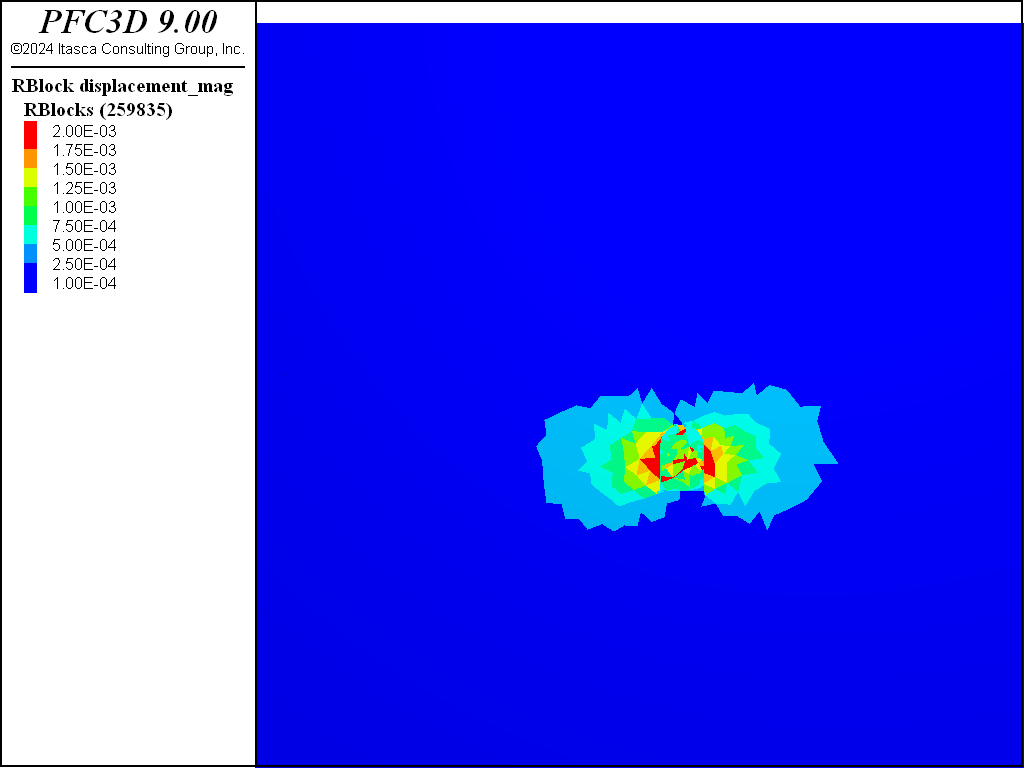
Figure 3: Displacement magnitude after the first stage of excavation.
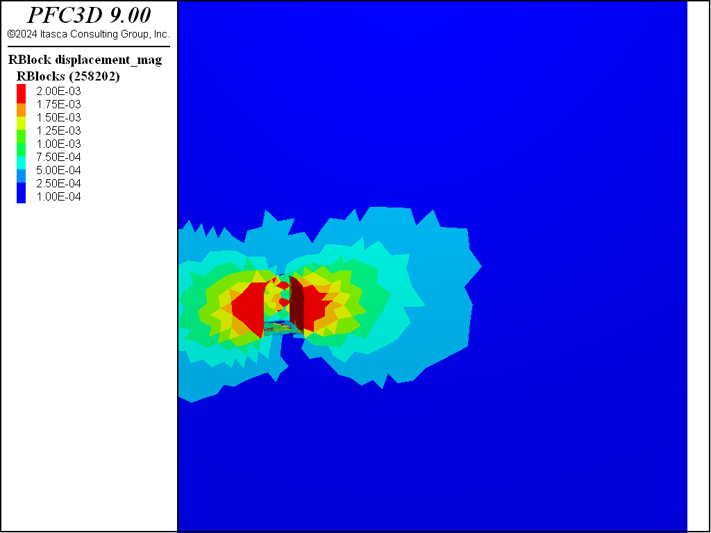
Figure 4: Displacement magnitude after the second stage of excavation.
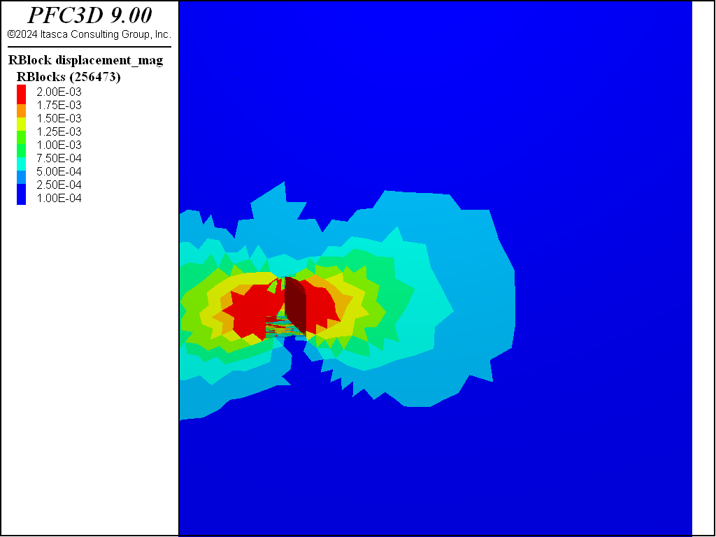
Figure 5: Displacement magnitude after the third stage of excavation.
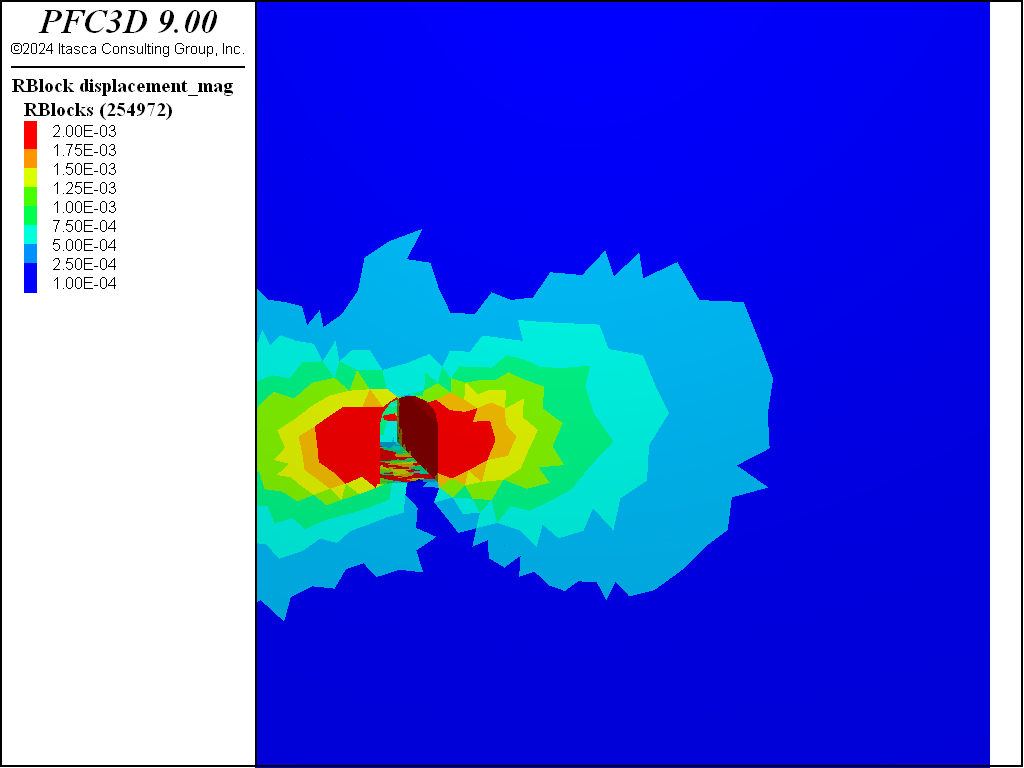
Figure 6: Displacement magnitude after the fourth stage of excavation.
The figures below show the evolution of minimum and maximum principal stresses after each stage of excavation. Note that the stages happen in 2 meter increments starting from -5 m. These plots correspond to the stresses inside the model at position 0, or 5 m from the initial tunnel face. The stress state at this location is largely unchanged from the initial stress state after the first stage of excavation (i.e., with excavation ending 3 m ahead of the plot location). After the second stage, corresponding to excavation to within 1 meter of the plot location, one can see noticeable differences in the stress state. The minimum principal stress increases ahead of the tunnel face footprint while the maximum principal stress decreases. There is a noticeable increase in the maximum principal stress above and horizontal of the tunnel opening. As the excavation progresses through the region the stresses continue to change with lobes of increasing and decreasing stresses. Note that in the plots purple colors are tensile stresses.
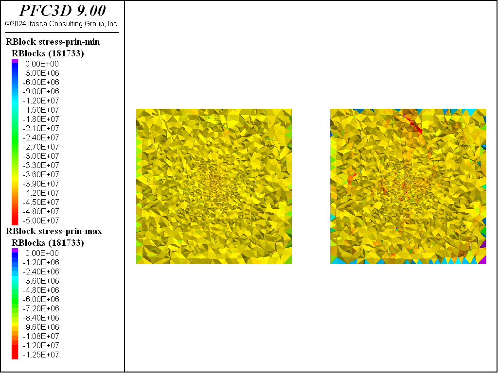
Figure 7: Minimum and maximum principal stresses after the first stage of excavation 5 m from the initial tunnel face.
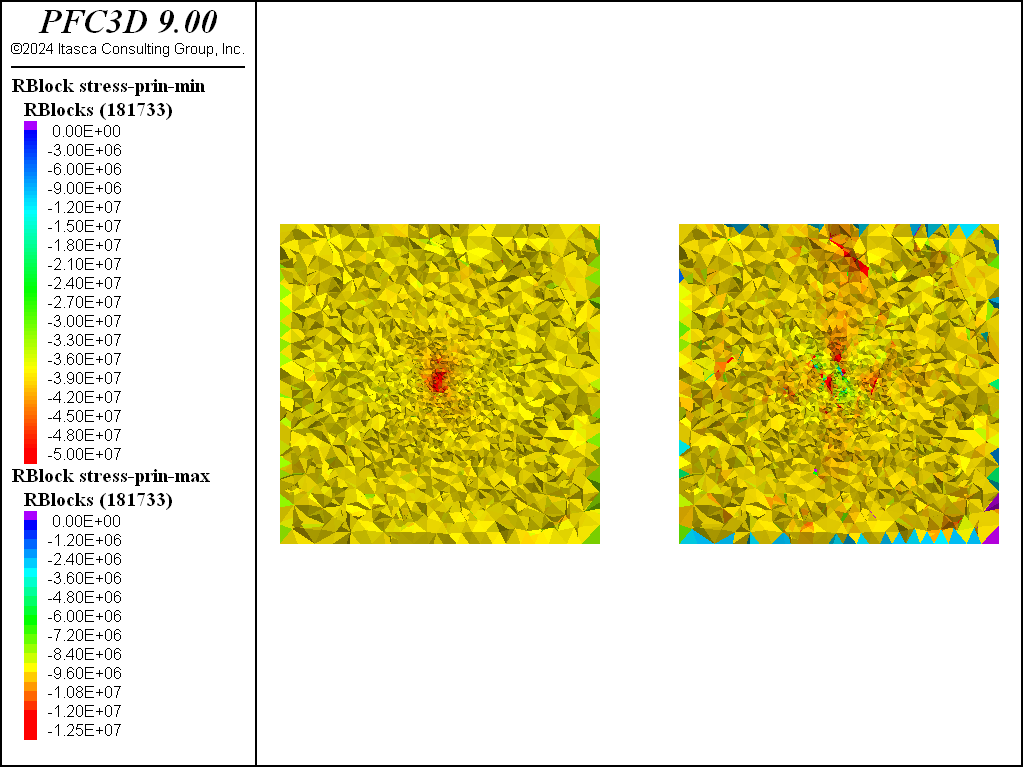
Figure 8: Minimum and maximum principal stresses after the second stage of excavation 5 m from the initial tunnel face.
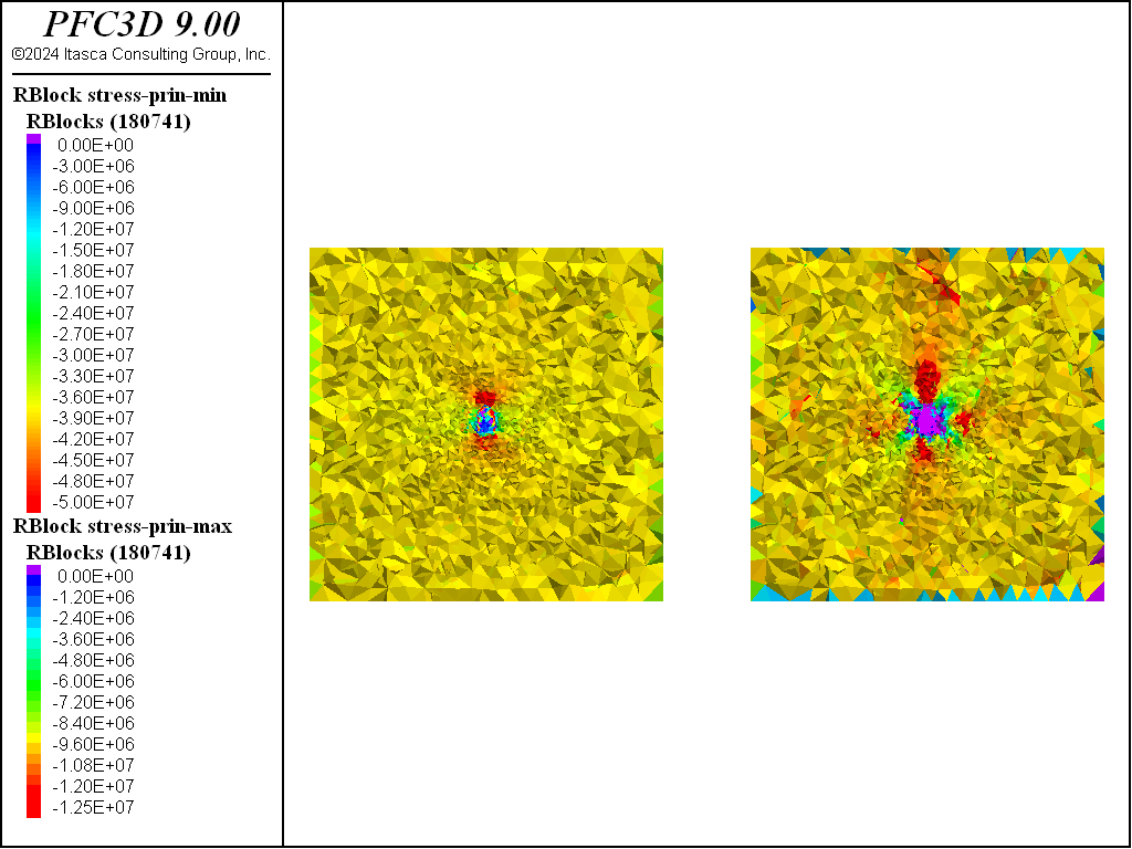
Figure 9: Minimum and maximum principal stresses after the third stage of excavation 5 m from the initial tunnel face.
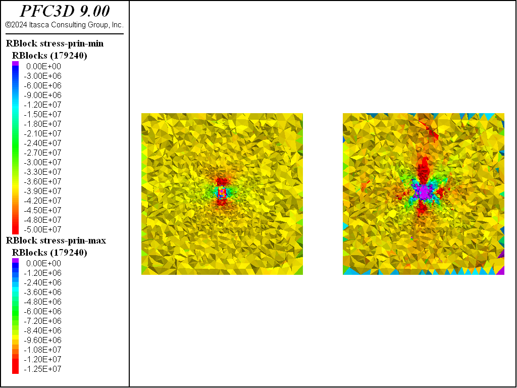
Figure 10: Minimum and maximum principal stresses after the fourth stage of excavation 5 m from the initial tunnel face.
The figure below shows the fragments for each stage of excavation. Note that any fragments formed in the tunnel faces from stages one through three are not shown. Fragments preferentially form on the lateral boundaries of the tunnel. A prominent fracture on the right of the model produces an obvious zone of fragmentation that is controlled by fracturing.
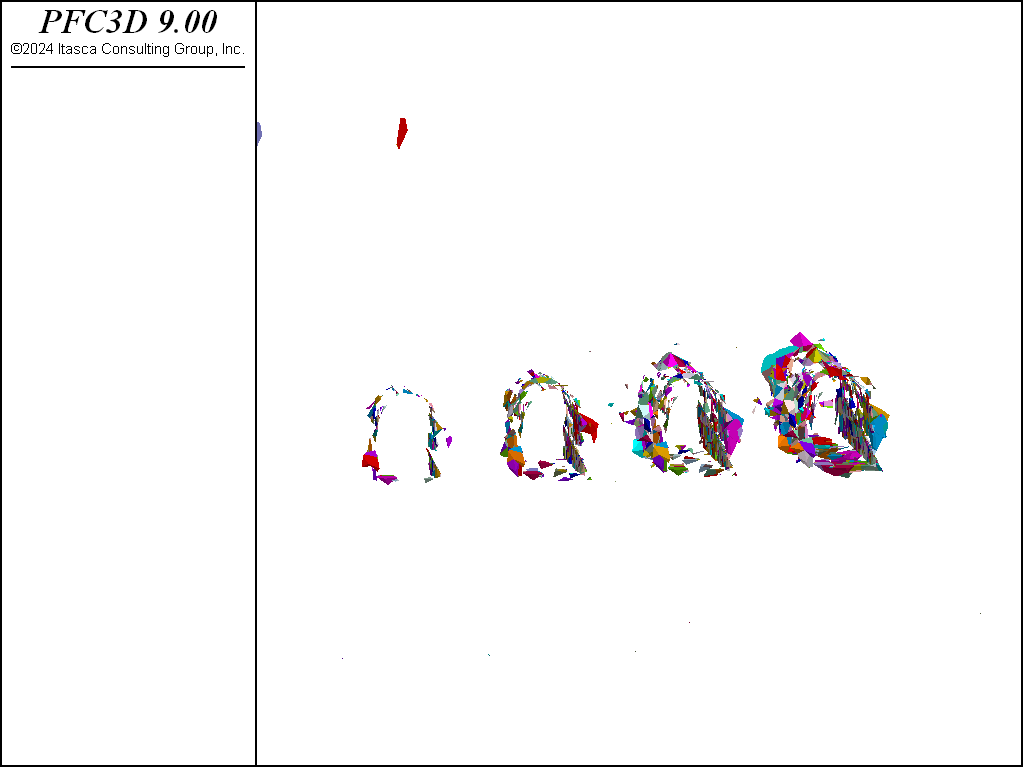
Figure 11: Fragments corresponding to each stage of excavation.
The final figures below show the progression of fracturing and slip on the faults for each stage of excavation. The maximum contour is the same as the displacement figures above. Slip is activated on a few large fractures, with some slip extending on the largest fractures to about twice the tunnel radius or more, with some limited slip on preferentially oriented fractures away from the tunnel.
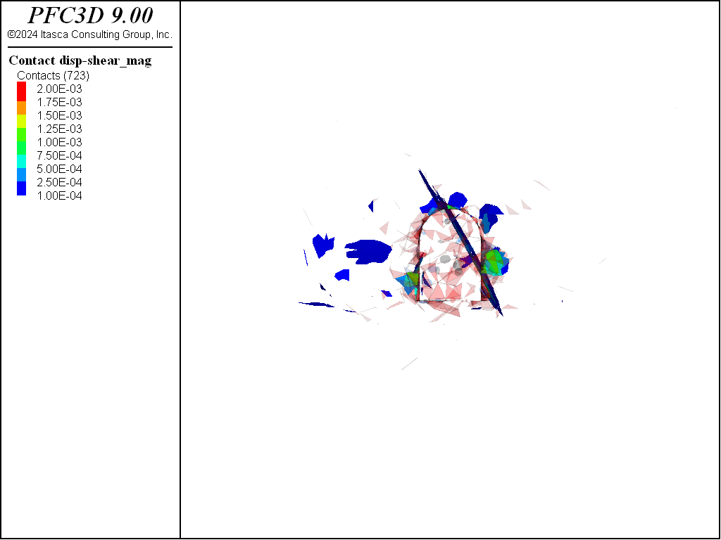
Figure 12: Fractures along with fault shear slip after the first stage of excavation.
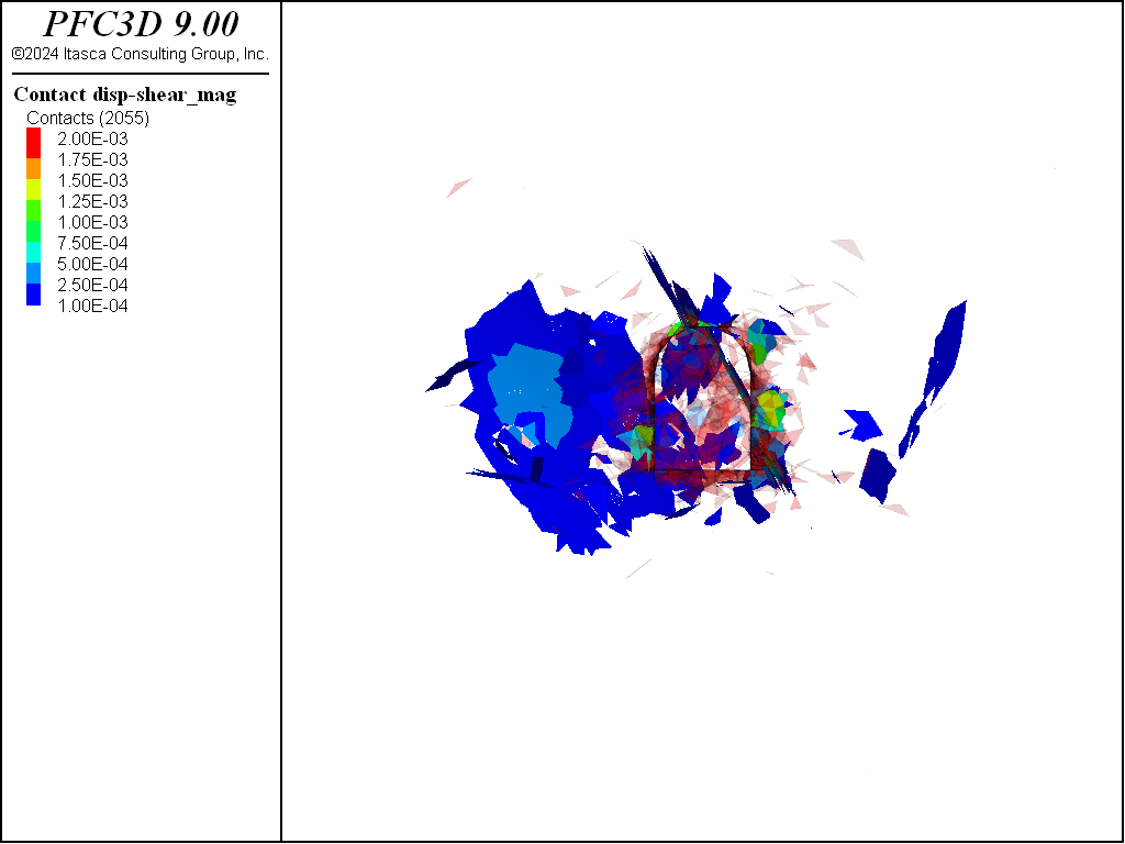
Figure 13: Fractures along with fault shear slip after the second stage of excavation.
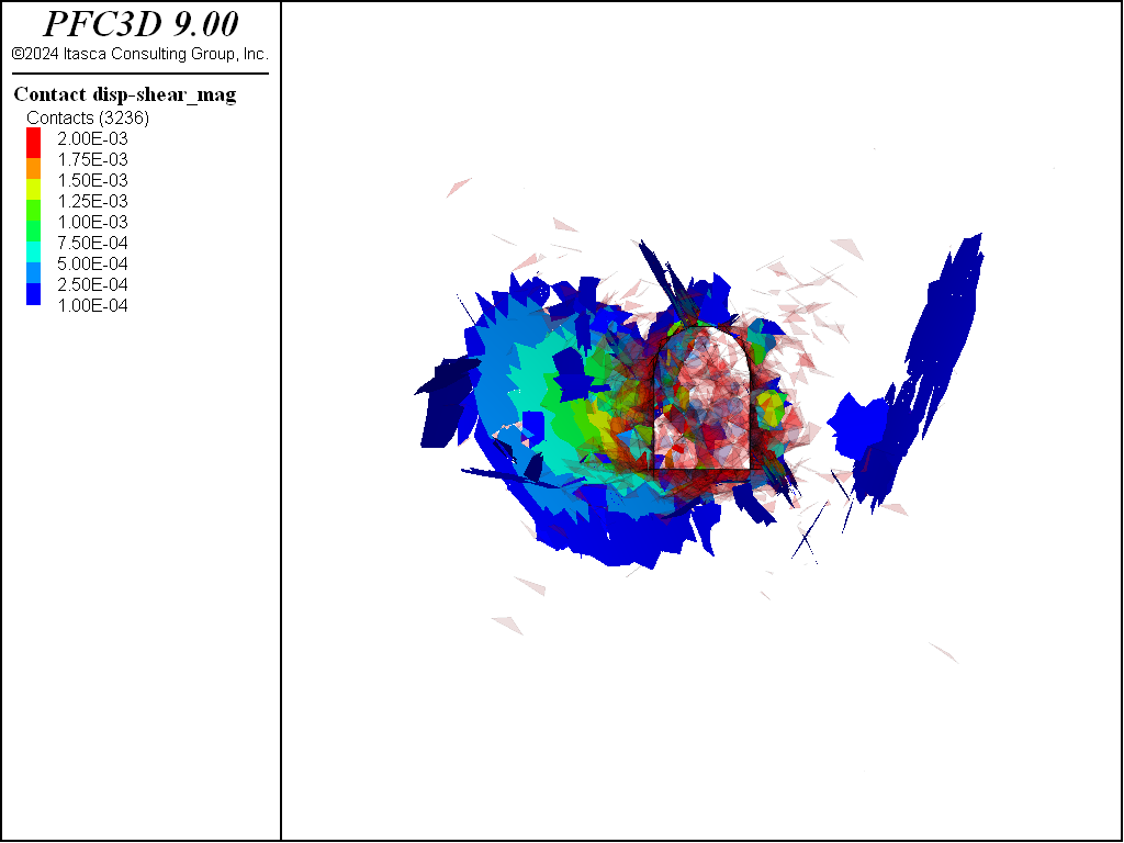
Figure 14: Fractures along with fault shear slip after the third stage of excavation.
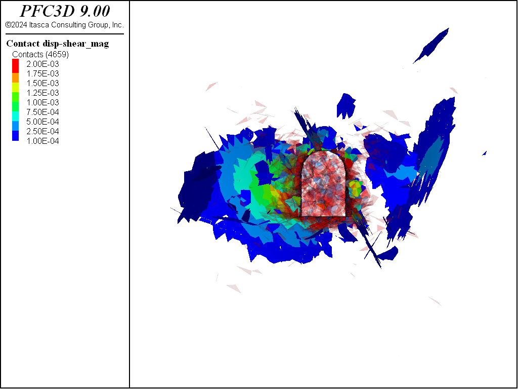
Figure 15: Fractures along with fault shear slip after the fourth stage of excavation.
Endnotes
Data Files
geometry.dat
; Create the rigid block geometry. Initially this will just
; be a tetrahedral packing that will later be cut.
model new

; Set the random seed so we get the same results each time
model random 10000

; Define the outer boundary and the specimen boundary for
; the excavation sequence
[boundLb = vector(-20,-5,-20)]
[boundUb = vector(20,20,20)]
[specLb = vector(-5.,-5,-5.)]
[specUb = vector(5.,5,5.)]
[spacing = 2]

; Specify the domain extent to be slightly larger than the boundary
model domain extent [boundLb->x-1] [boundUb->x+1] ...
                    [boundLb->y-1] [boundUb->y+1] ...
                    [boundLb->z-1] [boundUb->z+1]

; Create a geometry set to construct rigid blocks to fill the
; interior of the set.
geometry set 'blocks'
geometry generate box [boundLb->x] [boundUb->x] ...
                      [boundLb->y] [boundUb->y] ...
                      [boundLb->z] [boundUb->z]

; Make geometry nodes throughout the box and give them
; weights (as extra variables) to construct the rblock tetrahedra.
; This will help to eliminate the crystaline mesh using the INTERNAL keyword.
; In this case the sizes of the tets are scaled from the center of the model
[maxEdge = 0.5]
geometry fill [maxEdge]
geometry node extra 1 [maxEdge]
fish define addExtra
    local spacing = maxEdge
    local std = spacing/3
    local inMiddle = maxEdge
    local radius = 3.0
    local gs = geom.set.find("blocks")
    loop foreach local gn geom.node.list(gs)
        local pos = geom.node.pos(gn)
        if math.abs(pos->y) <  specUb->y+1
            pos->y = 0
        endif
        local factor = inMiddle+math.mag(pos)/radius*(1-inMiddle)
        local val = (math.random.uniform() - 0.5)*2.0*std*factor + math.max(spacing,spacing*factor)
        maxEdge = math.max(maxEdge,val)
        geom.node.extra(gn,1) = val
    endloop
end
[addExtra]
rblock construct from-geometry 'blocks' maximum-edge [maxEdge] internal
geometry delete

; Define groups on the boundaries. This should be done before scaling
rblock facet group 'x' slot 'boundary-x' range position-x [boundLb->x]
rblock facet group 'x' slot 'boundary-x' range position-x [boundUb->x]
rblock facet group 'y' slot 'boundary-y' range position-y [boundLb->y]
rblock facet group 'y' slot 'boundary-y' range position-y [boundUb->y]
rblock facet group 'z' slot 'boundary-z' range position-z [boundLb->z]
rblock facet group 'z' slot 'boundary-z' range position-z [boundUb->z]

; Assign single group to all boundary rigid blocks - will be useful
rblock group 'boundary=boundary' range ...
        group 'boundary-x=x' by rblock-facet
rblock group 'boundary=boundary' range ...
        group 'boundary-y=y' by rblock-facet
rblock group 'boundary=boundary' range ...
        group 'boundary-z=z' by rblock-facet

; Import the tunnel geometry from a dxf file and cut the rigid blocks
geometry import 'tunnel.dxf'
fracture import from-geometry 'tunnel'
rblock cut fractures throughgoing sliver-remove false group-facets 'tunnel' slot 'tunnel'

; Put the tunnel blocks in a group
rblock group 'tunnel' range geometry-space 'tunnel' count odd
fracture delete
geometry delete

; Define the excavation rounds and cut the tunnel
fracture joint-set dip 90 origin 0 [specLb->y+spacing] 0 ...
                   spacing [spacing] ...
                   number [math.floor((specUb->y - specLb->y)/spacing)]
rblock cut fractures throughgoing sliver-remove false ...
                     group-facets 'excavationSurf' slot 'excavationSurf' ...
                    range group 'tunnel'
fracture delete

; Create fractures throughout the volume and cut the rigid blocks. Do not cut the
; boundary rigid blocks
fracture template create "dfn-template" size power-law 3 size-limits 0.5 20
fracture generate dfn "dfn1" template "dfn-template" fracture-count 10000
rblock cut fractures throughgoing sliver-remove false group-facets 'cut' slot 'cut' ...
    range group 'boundary=boundary' not

; Define groups for the excavation surface for support force application
fish define defineExcavationSurf
    loop local i(1,math.floor((specUb->y - specLb->y)/spacing))
        local startY = specLb->y + (i-1)*spacing
        local endY = startY + spacing
        local gpname = "s" + string(i)
        io.out(startY)
        io.out(endY)
        command
            rblock facet group [gpname] slot 'support' range ...
                group 'tunnel' slot 'tunnel' ...
                position-y [startY] [endY]
            rblock facet group [gpname] slot 'support' range ...
                group 'excavationSurf' ...
                position-y [endY]
        endcommand
    endloop
end
[defineExcavationSurf]

; Scale the rigid blocks so that they overlap
rblock dilate expand 1e-5 relative keep-inertial

; Save the model
model save 'BBM_Geometry'
stress.dat
; Install the initial stress state in the specimen.

; Restore the initial geometry created in the previous step.
model restore 'BBM_Geometry'

; Specify the material properties. The SimpleBBM example
; can be used to calibrate a specimen.
[density = 2650.0]
[young = 50.0e9]
[poisson = 0.25]
[tensileStrength = 1.e7]
[cohesionFactor = 2.4]
[fricAngle = 35]

; Set the rigid block damping and density
rblock attribute density [density] damp 0.7

; Use the contact area, accumulate stress and deal with vertex-vertex
; and edge-edge contacts
rblock contact-resolution update-area true accumulate-stress true ...
                          facet-total 0.05 check-on-remap true

; Specify the subspringnetwork model properties. Initially
; all bonded contacts have infinite strength. This is
; useful when equilibrating the model.
contact cmat default model subspringnetwork method compute-stiffness ...
                           emod [young] poisson [poisson] ...
                           property sn_ten 1e100 sn_coh 1e100 ...
                           sn_fa [fricAngle] sn_cntconv 10 ...
                           fric [math.tan(fricAngle/180*math.pi)]

; Create contacts
model clean all

; No reason to detect contacts since in small strain
contact detection off type rblock-rblock

; Assign Weibull distribution for strength with constant cohesion-to-
; tensile ratio. The scale factor is fixed at 2.5.
fish define WeibullDist(c,mean,sfac,lcohFac)
    local ranNum= math.random.uniform
    ranNum = math.max(ranNum,0.0001)
    ranNum = math.min(ranNum,0.9999)
    local ten = mean*(-1.*math.ln(1.-ranNum))^(1./sfac)
    WeibullDist = ten
    contact.prop(c,'sn_coh') = ten * lcohFac
end
contact property sn_ten WeibullDist [tensileStrength] 2.5 [cohesionFactor] ...
    range group 'boundary=boundary' matches 1 not

; Identify the fracture contacts and assign the mohr model
contact group 'dfn1' range dfn 'dfn1' distance 0.1 orientation on ...
    group 'boundary=boundary' matches 1 not
contact model mohr range group 'dfn1'
contact property stiffness-normal 1e10 stiffness-shear 1e10 friction 30 cohesion 0 tension 0 ...
  range group 'dfn1'

; Keep a fixed area with the mohr model
contact method area

; Bond the subspringnetwork contacts
contact method bond gap -1000 1000

; Install stresses at all contacts. This must be done after the contacts are in
; place
rblock tractions constant -40e6 -30e6 -10e6 0 0 0

; Small strain with a timestep of 1 - quasi static conditions.
model mechanical timestep scale
model large-strain off

; Average ratio used in these simulations
[avgRatio = 1e-6]

; Fix the boundaries and solve elastically
rblock fix velocity-x spin-y spin-z range group 'x' slot 'boundary-x' by rblock-facet
rblock fix velocity-y spin-x spin-z range group 'y' slot 'boundary-y' by rblock-facet
rblock fix velocity-z spin-x spin-y range group 'z' slot 'boundary-z' by rblock-facet
model solve elastic only ratio-average [avgRatio] cycles 10 and

; Solve again allowing for breakage/slipping
model solve ratio-average [avgRatio] cycles 10 and

; Reset the displacement and shear displacement
rblock attribute displacement 0 0 0
contact property disp-shear 0 0 0

; Don't check for the convergence condition inside the specimen boundary
rblock extra 1 -1 range position [specLb] [specUb]

; Save the equilibrated model
model save 'BBM_Equil'
excavate.dat
; Cut out the tunnel

; Restore the equilibrated model
model restore 'BBM_Equil'

; Track the cracks
[broken = 0]
[tensileBreaks = 0]
[shearBreaks = 0]
[mixedBreaks = 0]
[shearNetwork = dfn.create("shear1")]
[tensileNetwork = dfn.create("tensile1")]
[mixedNetwork = dfn.create("mixed1")]
fish define onBondBroken(arr)
    local con = arr(1)
    local mode = arr(2)
    broken += 1
    if mode == 3
        fracture.from.contact(tensileNetwork,con)
        tensileBreaks += 1
    else
        if mode == 6
            fracture.from.contact(shearNetwork,con)
            shearBreaks += 1
        else
            fracture.from.contact(mixedNetwork,con)
            mixedBreaks += 1
        endif
    endif
end
fish callback add onBondBroken event bond_broken

; Record the number of breakages
fish history broken
fish history tensileBreaks
fish history shearBreaks
fish history mixedBreaks

; Ramp function for reduction of support stress
[rampCycles = 1000]
[preCycles = 500]
fish define computeFactor(rb,cyc)
    computeFactor = 1.0
    if cyc > preCycles
        computeFactor = 0.0
        local num = cyc - preCycles
        if num <= rampCycles
            computeFactor = 1-num/rampCycles
        endif
    endif
end

; Area of the tunnel to compute the average stress
fish define getArea(rblist,gp,slot)
    local ret = 0
    loop foreach local rb rblist
        loop local i(1,rblock.facet.num(rb))
            if rblock.facet.isgroup(rb,i,gp,slot)
                ret += rblock.facet.area(rb,i)
            endif
        endloop
    endloop
    getArea = ret
end

; Set up for the first excavation
rblock delete range group 'tunnel' position-y -5 -3
rblock group 'his=his1' range group 'support=s1' by rblock-facet
rblock extra 1 -1 range group 'his=his1'
[rblist = rblock.group.list('his1','his')]
[area = getArea(rblist,'s1','support')]
fish define appliedStress
    local v = 0
    loop foreach local rb rblist
        if rb # null
            v += math.mag(rblock.force.app(rb))
        endif
    endloop
    appliedStress = v/area
end
fish history appliedStress

; Excavate the first round
rblock facet apply unbalanced computeFactor range group 'support=s1'
model solve ratio-average [avgRatio] cycles [preCycles+rampCycles] and
fragment register rblock-rblock persist off
fragment compute group-slot 'excavate1'
model save 'excavate1'

; Excavate the second round
[shearNetwork = dfn.create("shear2")]
[tensileNetwork = dfn.create("tensile2")]
[mixedNetwork = dfn.create("mixed2")]
rblock delete range group 'tunnel' position-y -3 -1
rblock group 'his=his2' range group 'support=s2' by rblock-facet
[rblist = rblock.group.list('his2','his')]
[area = getArea(rblist,'s2','support')]
rblock facet apply-remove range group 'support=s1'
rblock facet apply unbalanced computeFactor range group 'support=s2'
model solve ratio-average [avgRatio] cycles [preCycles+rampCycles] and
fragment compute group-slot 'excavate2'
model save 'excavate2'

; Excavate the third round
[shearNetwork = dfn.create("shear3")]
[tensileNetwork = dfn.create("tensile3")]
[mixedNetwork = dfn.create("mixed3")]
rblock delete range group 'tunnel' position-y -1 1
rblock group 'his=his3' range group 'support=s3' by rblock-facet
[rblist = rblock.group.list('his3','his')]
[area = getArea(rblist,'s3','support')]
rblock facet apply-remove range group 'support=s2'
rblock facet apply unbalanced computeFactor range group 'support=s3'
model solve ratio-average [avgRatio] cycles [preCycles+rampCycles] and
fragment compute group-slot 'excavate3'
model save 'excavate3'

; Excavate the fourth round
[shearNetwork = dfn.create("shear4")]
[tensileNetwork = dfn.create("tensile4")]
[mixedNetwork = dfn.create("mixed4")]
rblock delete range group 'tunnel' position-y 1 3
rblock group 'his=his4' range group 'support=s4' by rblock-facet
[rblist = rblock.group.list('his4','his')]
[area = getArea(rblist,'s4','support')]
rblock facet apply-remove range group 'support=s3'
rblock facet apply unbalanced computeFactor range group 'support=s4'
model solve ratio-average [avgRatio] cycles [preCycles+rampCycles] and
fragment compute group-slot 'excavate4'
model save 'excavate4'
Endnotes
| Was this helpful? ... | Itasca Software © 2024, Itasca | Updated: Apr 02, 2024 |
