Genesis and Testing of a Soft-Bonded Material

	Example Resources
Data Files	Project: open “SoftBonded.prj”[1] in PFC3D

Problem Statement

The following example illustrates genesis and testing of a bonded-particle model using the Soft-Bond contact model. The system composed of balls is first generated in a periodic domain, then settled under low confining stress. This is achieved by distorting the periodic domain dimensions in order to achieve the prescribed stress state, using a servo-algorithm implemented as a FISH function. The soft-bond contact model is then installed at existing contacts, while the contact forces are reset. From this initial, stress-free system, the following tests are performed: a direct tension test, an unconfined compression test and a confined compression test. The methodologies used at each stage of the modeling process are discussed, and the response of the material is investigated.

Numerical Model

Specimen Genesis

The initial packing is generated by calling the file make_brick.dat, which uses the FISH functions defined in servo.fis. The specimen is generated in the entire model domain, with periodic boundary conditions in all directions, to avoid boundary effects. The function servo_domain implements the servo-control algorithm procedure, which aims at updating the domain extent in each direction in order to achieve and maintain a prescribed stress. The stress in the specimen is monitored using a measurement sphere. Note that this sphere is extended to encompass the entire domain, and the value of the stress that it computes is scaled to use the actual volume of the domain.

At this stage, the objective is to generate a dense, well connected packing. Since the contact model and properties will be overridden in a subsequent stage, a simple linear contact model is used. The friction coefficient is set to zero, and the deformability of the contacts is set to a value reasonably large with respect to the prescribed target stress, to optimize the computation time while preventing large overlaps. Note that increasing the target stress, or using frictional contacts would modify the geometry of the packing, and therefore its subsequent behavior.

The file make_brick.dat is partially parameterized for convenience. The file doall_A10.dat demonstrates how it can be executed, and the parameters chosen in this example:

model random 10001
[resolution = 10]   ; approx. number of balls accross specimen width 
[davg  = 2.5e-3]    ; average ball diameter (m)
[dratio = 1.66]     ; ball max/min diameter ratio [-]
[tag = 'A'+ string(resolution)]
program call 'make_brick.dat' 

The average ball diameter is set to 2.5mm, with a maximum to minimum diameter ratio of 1.66, to prevent local arrangement of the balls into crystalline structures. The parameter resolution used in this example denotes the target number of balls across the lateral dimension of the specimen, which is set to have a 2:1 aspect ratio.

Contact Model and Properties

Once the initial packing has been created, the file bond_sb.dat is used to install the soft-bond contact model and prepare the specimen for further testing. The contact forces are reset to zero, as well as the translational and rotational velocities of the balls and their accumulated forces/moments and displacements, and the contact model is replaced with the soft-bond model. Please refer to the documentation of this contact model for a detailed description of its behavior and properties.

The file bond_sb.dat is partially parameterized for convenience. The file doall_A10.dat demonstrates how it can be executed, and the parameters chosen in this example follow:

; Install contact model
model restore [string.build('brick_%1-iso',tag)]
[igap     = 0.0*davg ] 
[emod     = 50.0e9   ]
[kratio   = 2.5      ]
[fric     = 0.5      ]
[ten_mean = 20.0e6  ]
[ten_std  = 0.0e6    ]
[coh_mean = 100.0e6  ]
[coh_std  = 0.0e6    ]
[soft     = 0.0      ]
[cut      = 1.0      ]
[tag += '_G0_E50_KR25_S0_C1']
program call 'bond_sb.dat' 

The contact effective modulus is set to 50GPa, with a normal-to-shear stiffness ratio of 2.5 and a friction coefficient of 0.5. The contact tensile strength is set to 20MPa and the cohesion to 100MPa. Note that although the file bond_sb.dat is set to allow for a normal distribution of the strength parameters to be set, this functionality is not used in this example and all contacts are assigned the same strength parameters. Finally, the softening coefficient is set to 0.0 and the softening tensile strength factor is set to unity. With these values, softening is prohibited, and the model behaves essentially similar to the linear parallel-bond contact model with respect to failure.

Direct Tension Test

Two methods to simulate a direct tension test are described and compared below. The first method identifies balls on the two opposite ends of the specimen in the vertical direction, and fixes their velocity. The second method distorts the domain outward in the vertical direction.

Method 1: Using Ball Fixity

The file tt.dat is used to perform the direct tension test by fixing the velocities of a top and a bottom layer of balls. It is partially parameterized for convenience, and the file doall_A10.dat demonstrates how it can be executed, and the parameters chosen in this example follow:

; Perform Direct Tension Tests
[tag = 'A10_G0_E50_KR25_S0_C1']
model restore [string.build('brick_%1-bonded',tag)]
[strain_rate = 1.0]
[tag += '_SR1']
program call 'tt.dat'
[tag = 'A10_G0_E50_KR25_S0_C1']
model restore [string.build('brick_%1-bonded',tag)]
[strain_rate = 0.1]
[tag += '_SR01']
program call 'tt.dat'

The test is performed twice, with different values of the prescribed strain-rate (1.0 and 0.1). The stress-strain responses are shown in the figures below.

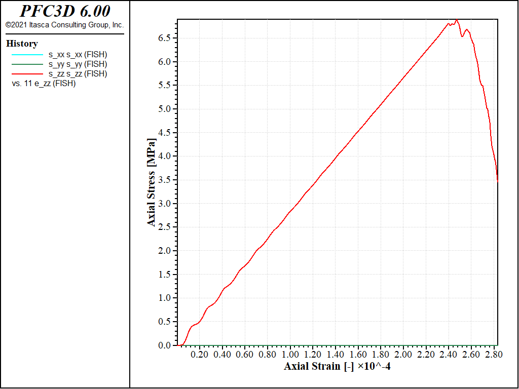
Figure 1: Stress vs Strain for a direct tension test with a strain rate of 1.0.

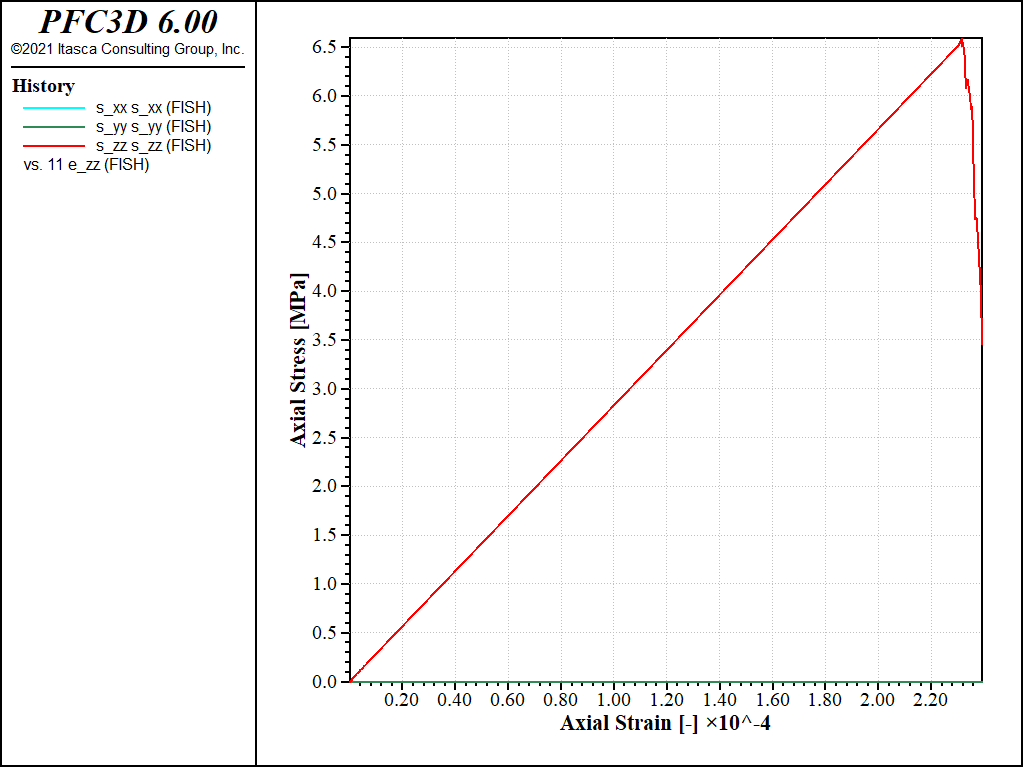
Figure 2: Stress vs Strain for a direct tension test with a strain rate of 0.1.

Both curves show the typical response of a brittle material, with a Young’s modulus of about 29GPa and a maximal tensile strength of about 8MPa in both cases. The strain rate has a small impact on the results: with the largest strain rate, the peak strength is slightly larger and reached at a slightly larger strain, with more pronounced oscillations at the beginning of the test.

Method 2: Using Domain Distortion

A similar test is performed by expanding the domain extent in the vertical direction. The file used to apply this test is tt2.dat, which is called by doall_A10.dat:

; Perform Direct Tension Test (using domain distortion)
[tag = 'A10_G0_E50_KR25_S0_C1']
model restore [string.build('brick_%1-bonded',tag)]
[strain_rate = 1.0]
[tag += '_SR1']
program call 'tt2.dat'

The stress-strain curve obtained in this case (strain-rate of 1.0) is shown in the figure below. The response agrees quantitatively well with that obtained with the first method (Figure 1)

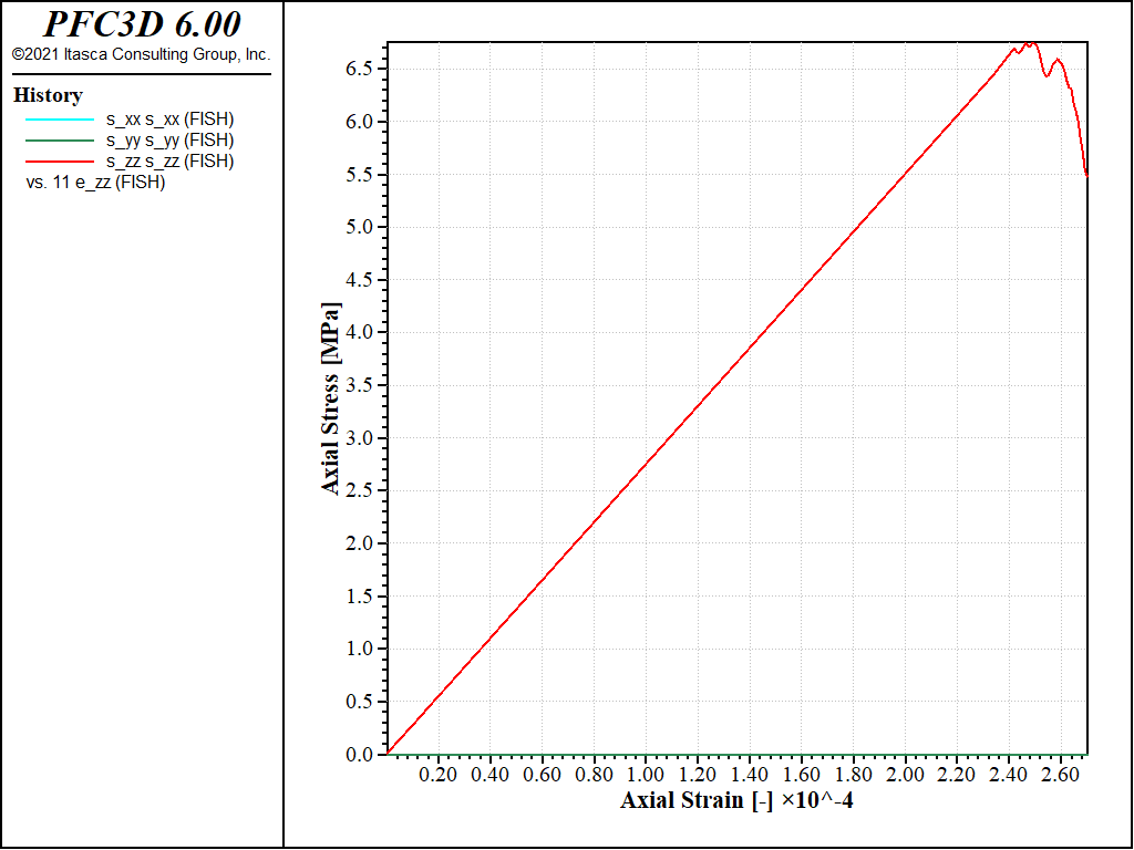
Figure 3: Stress vs Strain for a direct tension test with a strain rate of 1.0 (method 2).

Unconfined Compression Test

Two methods to simulate an unconfined compression test are described and compared below. The first method uses walls on the two opposite ends of the specimen in the vertical direction, and fixes their velocity. The second method distorts the domain inward in the vertical direction at a constant rate.

Method 1: Using Wall Platens

The file ucs.dat is used to perform the unconfined compression test using wall platens. It is partially parameterized for convenience, and the file doall_A10.dat demonstrates how it can be executed, and the parameters chosen in this example follow:

; Perform Unconfined Compression Test
[tag = 'A10_G0_E50_KR25_S0_C1']
model restore [string.build('brick_%1-bonded',tag)]
[strain_rate = 1.0]
[tag += '_SR1']
program call 'ucs.dat'
[tag = 'A10_G0_E50_KR25_S0_C1']
model restore [string.build('brick_%1-bonded',tag)]
[strain_rate = 0.1]
[tag += '_SR01']
program call 'ucs.dat'

The test is performed twice, with different values of the prescribed strain-rate (1.0 and 0.1). The stress-strain responses are shown in the figures below.

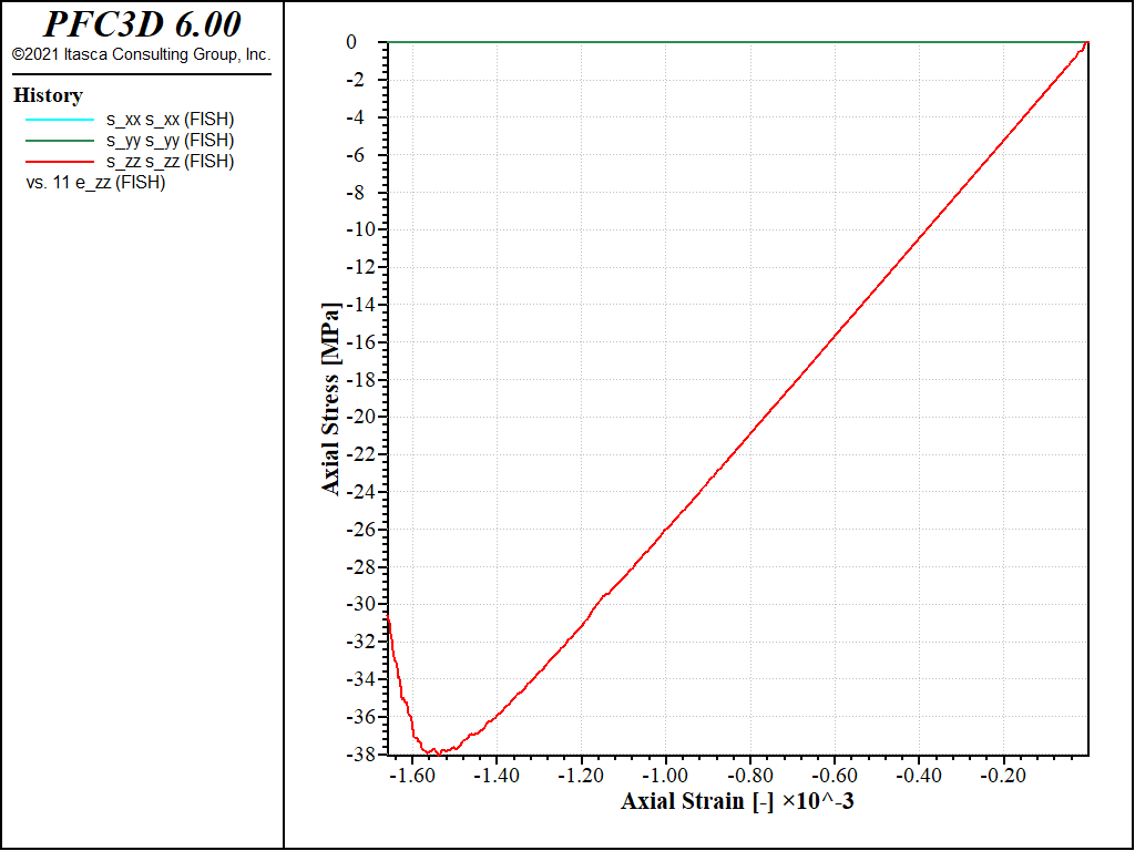
Figure 4: Stress vs Strain for an unconfined compression test with a strain rate of 1.0.

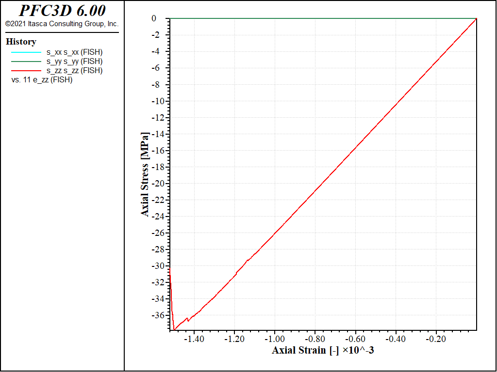
Figure 5: Stress vs Strain for an unconfined compression test with a strain rate of 0.1.

The peak compressive strength is about 32MPa, i.e. about 4 times the peak strength in tension, as typically observed for e.g. linear parallel-bonded models.

Method 2: Using Domain Distortion

A similar test is performed by contracting the domain extent in the vertical direction. The file used to apply this test is ucs2.dat, which is called by doall_A10.dat:

; Perform Unconfined Compression Test (using domain distortion)
[tag = 'A10_G0_E50_KR25_S0_C1']
model restore [string.build('brick_%1-bonded',tag)]
[strain_rate = 1.0]
[tag += '_SR1']
program call 'ucs2.dat'

The stress-strain curve obtained in this case (strain-rate of 1.0) is shown in the figure below. The response agrees quantitatively well with that obtained with the first method (Figure 4)

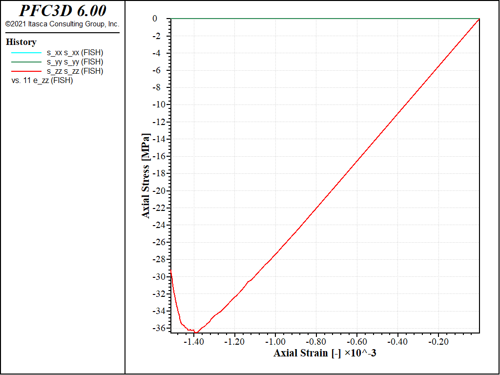
Figure 6: Stress vs Strain for an unconfined compression test with a strain rate of 1.0 (method 2).

Confined Compression Test

The file triax.dat is used to perform confined compression tests at various confining stress. It operates with periodic boundary conditions, and uses the servo-algorithm introduced above to apply the target confinement, then to maintain the lateral stress while contracting the specimen in the vertical direction at a constant strain-rate. It is partially parameterized for convenience, and the file doall_A10.dat demonstrates how it can be executed, and the parameters chosen in this example (strain-rate of 1.0 and a confining stress of 10kPa, 100kPa, 500kPa, 1MPa and 10MPa):

; Perform Confined Compression Tests
[tag = 'A10_G0_E50_KR25_S0_C1']
model restore [string.build('brick_%1-bonded',tag)]
[pc = -10.0e3]
[strain_rate = 1.0]
[tag = tag + '_P10_SR1']
program call 'triax.dat'
[tag = 'A10_G0_E50_KR25_S0_C1']
model restore [string.build('brick_%1-bonded',tag)]
[pc = -100.0e3]
[strain_rate = 1.0]
[tag = tag + '_P100_SR1']
program call 'triax.dat'
[tag = 'A10_G0_E50_KR25_S0_C1']
model restore [string.build('brick_%1-bonded',tag)]
[pc = -500.0e3]
[strain_rate = 1.0]
[tag = tag + '_P500_SR1']
program call 'triax.dat'
[tag = 'A10_G0_E50_KR25_S0_C1']
model restore [string.build('brick_%1-bonded',tag)]
[pc = -1000.0e3]
[strain_rate = 1.0]
[tag = tag + '_P1000_SR1']
program call 'triax.dat'
[tag = 'A10_G0_E50_KR25_S0_C1']
model restore [string.build('brick_%1-bonded',tag)]
[pc = -10000.0e3]
[strain_rate = 1.0]
[tag = tag + '_P10000_SR1']
program call 'triax.dat'

The stress-strain curves obtained are shown in the figure below, which shows a transition to a more ductile response at large confinement.

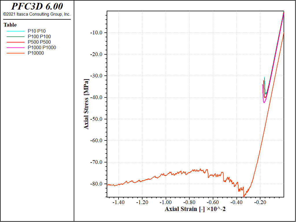
Figure 7: Stress vs Strain for an confined compression tests with a strain rate of 1.0 and increasing confinement.

Results and Discussion

The files discussed above demonstrate an effective set of procedures that can be used to generate a bonded-particle model, and perform direct-tension, unconfined compression and confined compression tests. In this example, the soft-bond contact model is used. The results shown above all use a set of parameters that forbid softening, and the resulting behavior has been shown to be that of a brittle material, with a compressive-to-tensile strength ratio of about 4.0, which is the value typically obtained with linear parallel-bonded materials, but is typically much low than the ratio most rocks exhibit.

A second set of tests is performed by executing the file doall_A10_S10_C0.dat. In this case, softening is activated by setting a value of 10.0 for the softening factor, and a value of 0.0 for the tensile strength softening factor. This means that once the tensile strength is reached at a specific contact, this contact enters a softening regime with a softening stiffness that is 1/10th of the loading stiffness, and breaks only if the tensile force reaches 0.0. The stress-strain curves obtained for a direct tension and unconfined compression tests are shown below.

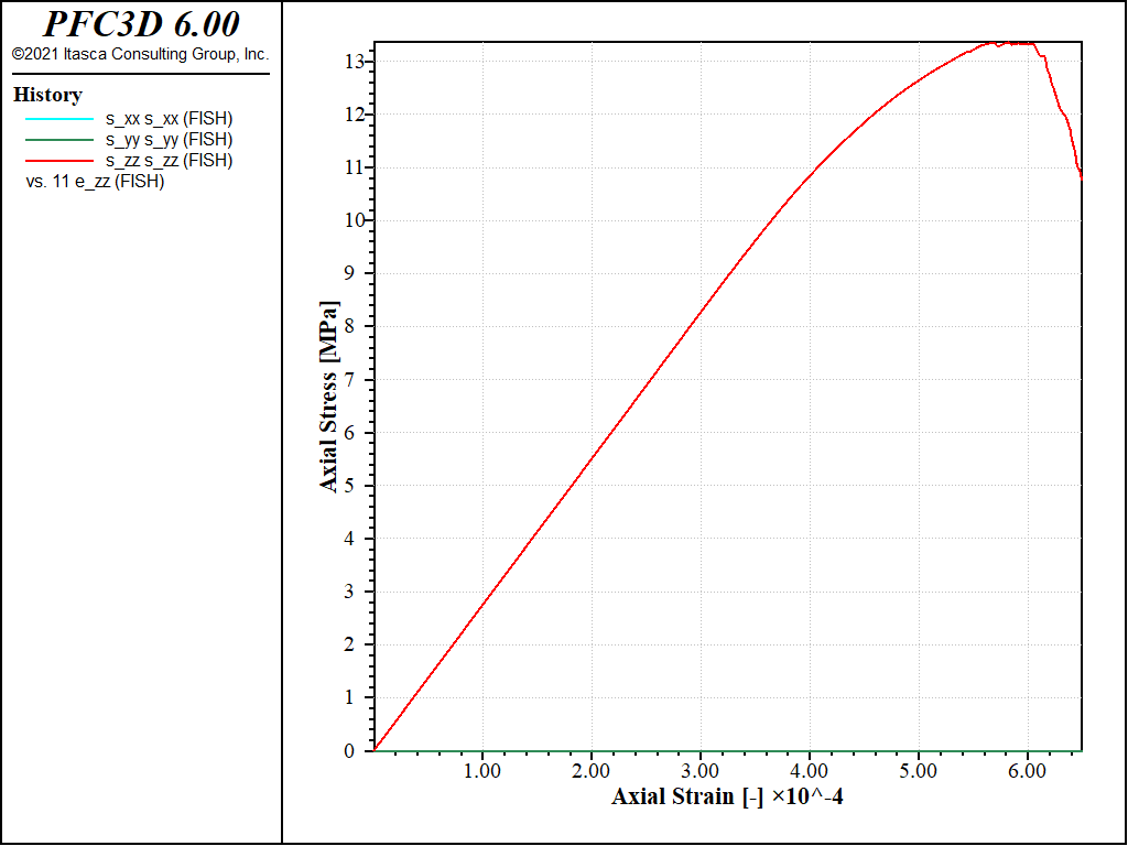
Figure 8: Stress vs Strain for a direct tension with a softening parameter of 10.

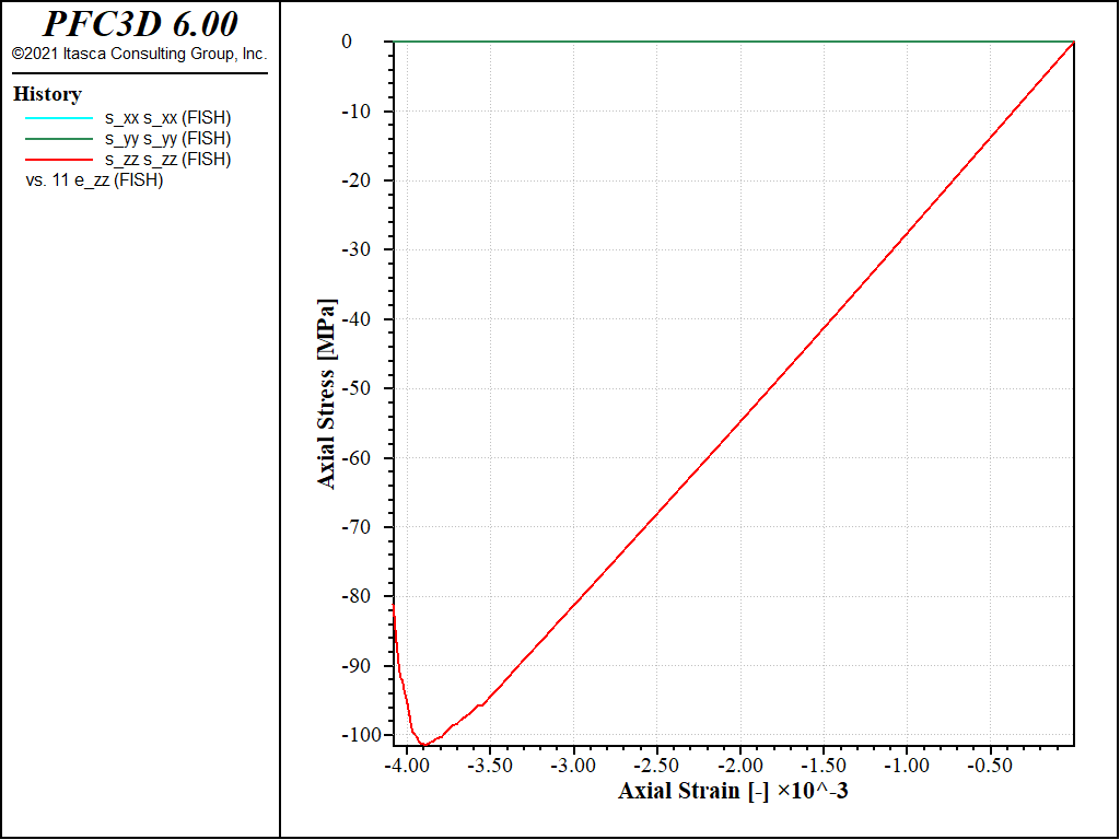
Figure 9: Stress vs Strain for an unconfined compression with a softening parameter of 10.

Under direct tension, the stress-strain curve exhibits a clear softening before reaching the peak strength, which is of about 14MPa (compared to 8MPa with no softening). Under compression, the peak strength is reached at about 100MPa, which leads to a compressive-to-tensile strength ratio of about 7.

A third set of tests is performed by executing the file doall_A10_S20_C0_COH1000.dat. In this case, softening is activated by setting a value of 20.0 for the softening factor, a value of 0.0 for the tensile strength softening factor, and the bond cohesion is increased to forbid shear failure.

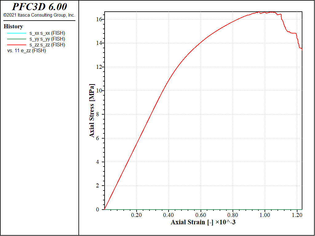
Figure 10: Stress vs Strain for a direct tension with a softening parameter of 20 and no shear failure allowed.

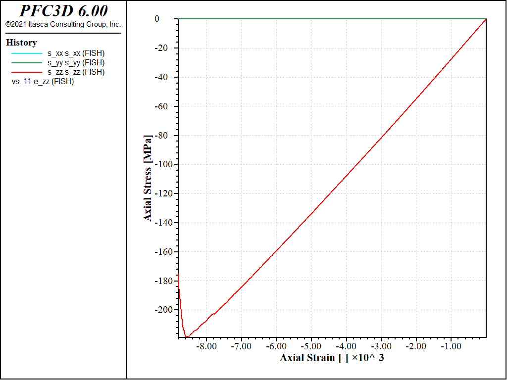
Figure 11: Stress vs Strain for an unconfined compression with a softening parameter of 20 and no shear failure allowed.

With these parameters, the peak strength increases to a value of about 200MPa in compression, and a value of about 17MPa in tension, i.e. a compressive-to-tensile strength ratio of about 12.0.

Endnote

[1]

This file may be found in PFC3D under the “example_applications/softbonded” folder in the Examples dialog (Help —> Examples on the menu). If this entry does not appear, please copy the application data to a new directory. (Use the menu commands Tools —> Copy App Data …. See the Copy Application Data section for details.)