Bilinear Strain-Softening/Hardening Ubiquitous-Joint (SUBI) Model
The bilinear strain-softening/hardening ubiquitous-joint (or, SUBI, for simplicity) model is a generalization of the ubiquitous-joint model. In the bilinear model, the failure envelopes for the matrix and joint are the composite of two Mohr-Coulomb model criteria with a tension cutoff that can harden or soften according to specified laws. A nonassociated flow rule is used for shear-plastic flow and an associated flow rule is used for tensile-plastic flow.
The softening behaviors for the matrix and the joint are specified in tables in terms of four independent hardening parameters (two for the matrix and two for the joint) that measure the amount of plastic shear and tensile strain, respectively. In this numerical model, general failure is first detected for the step, and relevant plastic corrections are applied. The new stresses are then analyzed for failure on the weak plane and updated accordingly. The hardening parameters are incremented if plastic flow has taken place, and the parameters of cohesion, friction, dilation, and tensile strength are adjusted for the matrix and the joint using the tables.
Formulations
Failure Criterion and Flow Rule for the Matrix
The criterion for failure in the matrix used in this model is sketched in the principal stress plane \(({\sigma}_1,{\sigma}_3)\) in Figure 1. (Recall that compressive stresses are negative and, by convention, \({\sigma}_1 \leq {\sigma}_2 \leq {\sigma}_3\).)
The failure envelope is defined by two Mohr-Coulomb failure criteria: \(f_2^s\) = 0 and \(f_1^s\) = 0 for segments \(A-B\) and \(B-C\), and a tension failure criterion \(f^t\) = 0 for segment \(C-D\).
The shear failure criterion has the general form \(f^s\) = 0. The criterion is characterized by a cohesion, \(c_2\), and a friction angle, \(\phi_2\), for segment \(A-B\), and by a cohesion, \(c_1\), and a friction angle, \(\phi_1\), for segment \(B-C\). The tensile failure criterion is specified by means of the tensile strength, \(\sigma^t\) (positive value); thus we have
where
Note that the tensile cap acts on segment \(B-C\) of the shear envelope and, for a material with nonzero friction angle \(\phi_1\), the maximum value of the tensile strength is given by
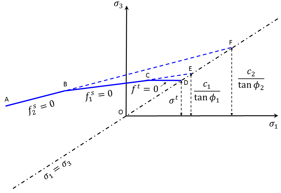
Figure 1: FLAC3D bilinear matrix failure criterion.
In the model formulation, elastic guesses for the stresses are first evaluated for the step using total strain increments. Plastic yielding is detected if the corresponding stress point \((\sigma_1^I,\sigma_3^I)\) lies outside the failure surface representation in Figure 1. In this case, a stress correction must be applied to the elastic guess. It is determined by allowing plastic flow to occur, in order to restore the condition \(f_2^s\) = 0, \(f_1^s\) = 0 or \(f^t\) = 0, depending on the position of the stress point above \(A-B\), \(B-C\), or \(C-D\). (Bisectors are used at \(B\) and \(C\) to delimit the domain of failure attached to a particular segment of the yield surface.)
The usual assumption is made that total strain increments can be decomposed into elastic and plastic parts. The flow rule for plastic yielding has the form
where \(i\) = 1,3. The potential function, \(g\), for shear yielding is \(g^s\). This function corresponds to the nonassociated law,
where \(\psi\), the dilation angle, is equal to \(\psi_2\) for failure along \(A-B\), and \(\psi_1\) along \(B-C\), and
The potential function for tensile yielding is \(g^t\). It corresponds to the associated flow rule,
The plastic strain increments for shear failure have the form
The stress corrections for shear failure are
where
and, by definition:
In turn, the plastic strain increments for tensile failure have the form
The stress corrections for tensile failure are
where
Failure Criterion and Flow Rule for the Weak Plane
The stresses, corrected for plastic flow in the matrix, are resolved into components parallel and perpendicular to the weak plane and tested for ubiquitous-joint failure. The failure criterion is expressed in terms of the magnitude of the tangential traction component, \(\tau = \sqrt{{{\sigma}_{1'3'}}^2 + {{\sigma}_{2'3'}}^2}\), and the normal traction component, \(\sigma_{3'3'}\), on the weak plane.
The failure criterion is represented in Figure 1 and corresponds to two Mohr-Coulomb failure criteria (\(f_2^s\) = 0 for segment \(A-B\), and \(f_1^s\) = 0 for segment \(B-C\)) and a tension failure criterion (\(f^t\) = 0 for segment \(C-D\)). Each shear criterion has the general form \(f^s\) = 0 and is characterized by a cohesion and a friction angle \(c_j, \phi_j\), equal to \(c_{j_2}, \phi_{j_2}\) along segment \(A-B\), and \(c_{j_1}, \phi_{j_1}\) along \(B-C\). The tensile criterion is specified by means of the tensile strength, \(\sigma_j^t\) (positive value). Thus, we have
Note that for a weak plane with nonzero friction angle \({\phi}_{j_1}\), the maximum value of the tensile strength is given by
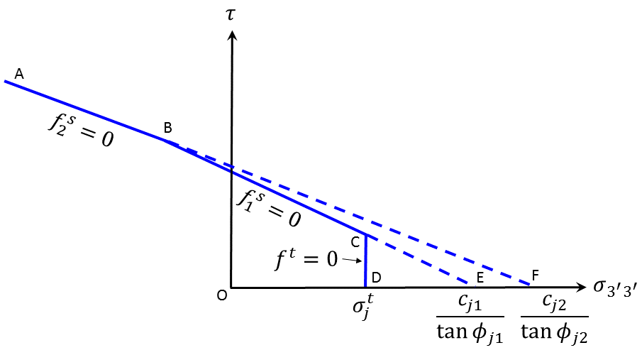
Figure 2: FLAC3D bilinear joint failure criterion.
Yield is detected and stress corrections are applied using a technique similar to the one described in the matrix context.
Here, the flow rule for plastic yielding has the form
where \(\gamma\) is the strain variable associated with \(\tau\), and we have
The potential function, \(g\), for shear yielding on the weak plane is \(g^s\). It corresponds to the nonassociated law,
where \(\psi_j\), the dilation angle, is equal to \(\psi_{j_2}\) for failure along \(A-B\), and \(\psi_{j_1}\) along \(B-C\).
The potential function \(g\) for tensile yielding on the weak plane is \(g^t\). It corresponds to the associated flow rule,
The local plastic strain increments for shear failure are such that
The stress corrections for shear failure are
where
and the superscript \(^O\) indicates values obtained just before detection of failure on the weak plane.
The plastic corrections for the local shear stress components on the weak plane are derived by scaling:
In turn, local plastic strain increments for tensile failure have the form
The stress corrections for tensile failure are
where
Large-Strain Update of Orientation
In large strain, the orientation of the weak plane is adjusted per zone to account for rigid-body rotations, and rotations due to deformations. The large-strain update to orientation is identical to those described in the ubiquitous-joint model.
Hardening Parameters
In the bilinear strain-softening/hardening ubiquitous-joint model, some or all of the
zone yielding parameters (i.e., cohesion, friction, dilation and tensile strength) for
the matrix and joint are modified automatically, after the onset of plasticity,
according to piecewise linear laws specified on input in terms of a range of values for
the hardening parameters. (See the section of
user-defined functions in the
strain-softening/hardening model.) One table number must be
specified in the zone property (FLAC3D) or block zone property (3DEC) command for each softening parameter. (If
no table property number is specified, the parameter is taken as constant.) The
corresponding table data contain pairs of values for the parameter and the property
between which a linear variation is assumed. The last property value is used for values
of the hardening parameter beyond the last one specified in the table.
Four independent hardening parameters are used in this model:
- \({\kappa}^s\) measures the matrix plastic shear strain and is used to update the matrix cohesion, friction, and dilation;
- \({\kappa}^t\) measures the matrix plastic volumetric tensile strain and is used to update the matrix tensile strength;
- \({\kappa}_j^s\) estimates the joint plastic shear strain and controls the joint cohesion, friction, and dilation update; and
- \({\kappa}_j^t\) evaluates the joint plastic volumetric tensile strain and controls the joint tensile strength update.
The parameters are defined as the sum of incremental measures of plastic strain for the zone. The zone-hardening increments are calculated as the volumetric average of hardening increments over all tetrahedra involved in the zone.
The shear-hardening increment for a tetrahedron is the square root of the second invariant of the incremental plastic shear-strain deviator tensor for the step. For the matrix, it is given as
where \(\Delta {\epsilon}_m^{p_s}\) is the mean plastic strain increment,
and the plastic strain increments are given by Equation (9), using Equation (11) for \({\lambda}^s\).
For the joint, the formula is
where the plastic strain increments are given by Equation (23) (see Equation (20)), using the form (25) for \({\lambda}^s\).
The tetrahedron tensile-hardening increment is the plastic volumetric tensile-strain increment.
For the matrix, we have
where the plastic strain increment is given by Equation (13), using Equation (15) for \({\lambda}^t\).
For the joint, the expression is
where the plastic strain increment is given by Equation (27), using the Equation (29) for \({\lambda}^t\).
Implementation Procedure
The implementation of the bilinear model in FLAC3D proceeds as indicated above. An elastic guess, \({\sigma}_{ij}^I\), is first computed using stress increments for the step evaluated by application of Hooke’s law to the total strain increments, \(\Delta {\epsilon}_{ij}\). Principal stresses are calculated, ordered such that \({\sigma}_1^I \leq {\sigma}_2^I \leq {\sigma}_3^I\), and tested for failure in the matrix using the yield criteria defined by Equation (1) and (2). In principle, matrix failure is declared if the representation of the stress point \((\sigma_1^I,\sigma_3^I)\) falls outside the yield surface in Figure 1. In this case, stress corrections are applied to the principal values of the elastic guess, which depend on the position of the stress point above \(A-B\), \(B-C\) or \(C-D\). (Bisectors are used at \(B\) and \(C\) to delimit the domain of failure attached to a particular segment of the yield surface.)
The stress corrections for shear failure in the matrix are given by Equations (10) and (11), where the parameters of cohesion, \(c\), friction, \(\phi\), and dilation, \(\psi\), have value \(c_2, \phi_2, \psi_2\) for failure along \(A-B\), and \(c_1, \phi_1,\psi_1\) for failure along \(B-C\).
The stress corrections for tensile failure in the matrix are given by by Equations (14) and (15).
The stress tensor components in the system of reference axes, \({\sigma}_{ij}^O\), are then calculated from the corrected principal values by assuming that the principal directions have not changed during plastic flow.
Local traction components on the weak plane are defined as \({\sigma}_{3'3'}\) and \(\tau\), with \({\sigma}_{3'3'}\) being the normal component, and \(\tau = \sqrt{{{\sigma}_{1'3'}}^2 + {{\sigma}_{2'3'}}^2}\) being the magnitude of the tangential traction component. (The local axis 1สน is in the dip direction, 2สน the strike, and 3สน the normal to the weak plane.) These stresses are resolved from \({\sigma}_{ij}^O\) and examined for ubiquitous-joint failure using the yield criteria (Equations (16) and (17)). In principle, ubiquitous-joint failure is declared if the representation of the stress point \((\sigma_{3'3'}^O,\tau^O)\) falls outside the yield surface in Figure 2. In this case, local stress corrections, which depend on the position of the stress point in the vicinity of \(A-B\), \(B-C\) or \(C-D\), are applied. (Bisectors are used at \(B\) and \(C\) to delimit the domain of failure attached to a particular segment of the yield surface.)
The stress corrections for shear joint failure are given by Equations (24) to (26), where the parameters of cohesion, \(c_j\), friction, \(\phi_j\), and dilation, \(\psi_j\), have values \(c_{j_2}, \phi_{j_2}, \psi_{j_2}\) for failure along \(A-B\), and \(c_{j_1}, \phi_{j_1}, \psi_{j_1}\) for failure along \(B-C\).
The stress corrections for tensile joint failure are given by Equations (28) and (29).
Finally, the local stress components are resolved back into global axes.
In large-strain mode, the unit normal to the weak plane is adjusted per zone to account for body rotations.
After determination of the new stresses for the step, the hardening parameters are incremented using Equations (30), (32), (33), and (34). These parameters are then used to determine new values of cohesion, friction, dilation and tensile strength for the matrix and the joint from the available input tables.
It is assumed that the tensile strength of the material can never increase. Also, for material with friction, the value will not exceed the maximum value \({\sigma}_{max}^t\) or \({{\sigma}_j^t}_{max}\) (see Equations (4) and (18)).
Note that, by default, the yield model is linear in both the matrix and the joint, in which case only sections 1 (where \(f_1^s\) = 0) and 3 (where \(f^t\) = 0) of the yield curve are recognized (even if properties are assigned for section 2, where \(f_2^s\) = 0). To activate the bilinear laws, the property flag-bilinear and/or the property flag-bilinear-joint must be set to 1.
Also, if the friction angles for sections 1 and 2 become equal, the model will be considered as linear, and section 2 will be ignored (for the matrix and/or the joint, as appropriate). Section 2 will also be ignored if the intersection of sections 1 and 2 corresponds to a stress point that violates the tensile criterion.
softening-ubiquitous model properties
Use the following keywords with the zone property (FLAC3D) or block zone property (3DEC) command to set these properties
of the bilinear strain-softening/hardening ubiquitous-joint model.
- softening-ubiquitous
- bulk f
elastic bulk modulus, \(K\)
- cohesion f
matrix cohesion, \(c\) = \(c_1\)
- cohesion-2 f
matrix cohesion, \(c_2\)
- dip f
dip angle [degrees] of weakness plane
- dip-direction f
dip direction [degrees] of weakness plane
- friction f
matrix friction angle, \(\phi\) = \(\phi_1\)
- friction-2 f
matrix friction angle, \(\phi_2\)
- poisson f
Poisson’s ratio, \(\nu\)
- shear f
elastic shear modulus, \(G\)
- young f
Young’s modulus, \(E\)
- joint-cohesion f
joint cohesion, \(c_j\) = \(c_{j1}\)
- joint-cohesion-2 f
joint cohesion, \(c_{j2}\)
- joint-friction f
joint friction angle, \(\phi_j\) = \(\phi_{j1}\)
- joint-friction-2 f
joint friction angle, \(\phi_{j2}\)
- normal v
normal direction of the weakness plane, (\(n_x\), \(n_y\), \(n_z\))
- normal-x f
\(x\)-component of the normal direction to the weakness plane, \(n_x\)
- normal-y f
\(y\)-component of the normal direction to the weakness plane, \(n_y\)
- normal-z f
\(z\)-component of the normal direction to the weakness plane, \(n_z\)
- flag-bilinear-joint i (a)
= 0 (default) for joint linear model ;
= 1 for joint bilinear model ;
< 0 joint effect will be skipped, so that the model is degenerated into a bilinear Mohr-Coulomb model.
- flag-brittle b (a)
If true, the tension limit is set to 0 in the event of tensile failure. The default is false.
- table-cohesion s (a)
name of the table relating matrix cohesion \(c\) = \(c_1\) to matrix plastic shear strain.
- table-cohesion-2 s (a)
name of the table relating matrix cohesion \(c_2\) to matrix plastic shear strain.
- table-dilation s (a)
name of the table relating matrix dilation angle \(\psi\) = \(\psi_{1}\) to matrix plastic shear strain.
- table-dilation-2 s (a)
name of the table relating matrix dilation \(\psi_{2}\) to matrix plastic shear strain.
- table-friction s (a)
name of the table relating matrix friction \(\psi\) = \(\psi_{1}\) angle to matrix plastic shear strain.
- table-friction-2 s (a)
name of the table relating matrix friction angle \(\psi_{2}\) to matrix plastic shear strain.
- table-joint-cohesion s (a)
name of the table relating joint cohesion \(c_j\) = \(c_{j1}\) to joint plastic shear strain.
- table-joint-cohesion-2 s (a)
name of the table relating joint cohesion \(c_{j2}\) to joint plastic shear strain.
- table-joint-dilation s (a)
name of the table relating joint dilation \(\psi_j\) = \(\psi_{j1}\) to joint plastic shear strain.
- table-joint-dilation-2 s (a)
name of the table relating joint dilation \(\psi_{j2}\) to joint plastic shear strain.
- table-joint-friction s (a)
name of the table relating joint friction angle \(\phi_j\) = \(\phi_{j1}\) to joint plastic shear strain.
- table-joint-friction-2 s (a)
name of the table relating joint friction angle \(\phi_{j2}\) to joint plastic shear strain.
- table-joint-tension s (a)
name of the table relating joint tension limit \(\sigma^t_j\) to joint plastic tensile strain.
- strain-shear-plastic f (r)
accumulated plastic shear strain
- strain-shear-plastic-joint f (r)
accumulated joint plastic shear strain
- strain-tensile-plastic f (r)
accumulated plastic tensile strain
- strain-tensile-plastic-joint f (r)
accumulated joint plastic tensile strain
Key
- (a) Advanced property.
- This property has a default value; simpler applications of the model do not need to provide a value for it.
- (r) Read-only property.
- This property cannot be set by the user. Instead, it can be listed, plotted, or accessed through FISH.
Notes
- Only one of the two options is required to define the elasticity: bulk modulus \(K\) and shear modulus \(G\), or, Young’s modulus \(E\) and Poisson’s ratio \(\nu\). When choosing the latter, Young’s modulus \(E\) must be assigned in advance of Poisson’s ratio \(\nu\).
- Only one of the three options is required to define the orientation of the weakness plane: dip and dip-direction; a norm vector (\(n_x, n_y, n_z\)); or, three norm components: \(n_x\), \(n_y\), and \(n_z\).
- The tension cut-off is \({\sigma}^t = min({\sigma}^t, c/\tan \phi)\).
- The joint tension limit used in the model is the minimum of the input \(\sigma^t\) and \({c_j}/{\tan \phi_j}\).
- The tension table and flag-brittle should not be active at the same time.
| Was this helpful? ... | 3DEC © 2019, Itasca | Updated: Feb 25, 2024 |