Boundary Conditions
The boundary conditions in a numerical model consist of the values of field variables (e.g., stress and displacement) that are prescribed at the boundary of the numerical grid. Boundaries are of two categories: real and artificial. Real boundaries exist in the physical object being modeled (e.g., a tunnel surface or the ground surface). Artificial boundaries do not exist in reality, but they must be introduced in order to enclose the chosen number of zones. The conditions that can be imposed on each type are similar; these conditions are discussed first. Then (in Artificial Boundaries) some suggestions concerning the location and choice of artificial boundaries and the effect they have on the solution are made.
Mechanical conditions that can be applied at boundaries are of two main types: prescribed displacement or prescribed stress. A free surface is a special case of the prescribed-stress boundary. The two types of mechanical conditions are described in Stress Boundary and Displacement Boundary.
All examples listed in this section can be found in the project file “BoundaryConditions.prj.”
Stress Boundary
By default, the boundaries of a FLAC3D grid are free of stress and any constraint. Forces or
stresses may be applied to any boundary, or part of a boundary, by means of the
zone face apply command. Individual components of the stress tensor are specified with
the stress-xx, etc., keywords. For example, the commands
zone face apply stress-zz -1e5 range position-z 0
zone face apply stress-xz -5e4 range position-z 0
apply the given \(\sigma_{zz}\) and \(σ_{xz}\) components of a stress tensor to all boundary zone faces with centroids that fall within the range -0.1 ≤ \(z\) ≤ 0.1. All other stress components are zero.
Stress can be applied either in the global model \(x\),\(y\),\(z\)-directions, or in directions normal and tangential to the local boundary face. The keyword stress-normal applies a normal stress to a face, while keywords stress-dip and stress-strike apply shear stresses to the face. stress-dip is the stress component applied in the dip direction of the local face, and stress-strike is the stress component applied in the strike direction. The orientation of the local face axes is illustrated in the next figure. Note that global (\(x\),\(y\),\(z\))-axes stresses and local (\(d\),\(s\),\(n\))-axes stresses cannot both be applied to the same face.
There are several things to note about this use of zone face apply command. First, only
those faces inside the range defined by range will be affected by the
zone face apply command, and as with all face selection geometric range elements, will
select by the location of the face centroid. Second, compressive stresses have a negative
sign, in accordance with the general sign convention for internal
stresses in FLAC3D. Finally, FLAC3D actually applies the stress components as forces, or
tractions, which result from a stress tensor acting on the given boundary plane; the tractions
are computed whenever a model solve command is issued, and again every tenth step in
large-strain mode.
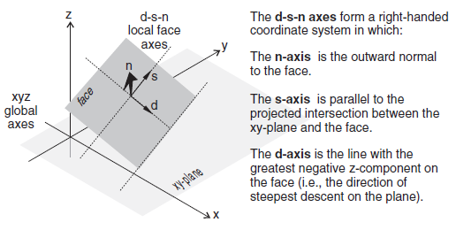
Figure 1: Local face axes defined by (d) dip direction, (s) strike direction, and (n) normal direction.
Individual forces can also be applied to the grid by using the zone gridpoint fix command
and the force-applied-x, force-applied-y, and force-applied-z keywords,
which specify the \(x\)-, \(y\)-, and \(z\)-components of an applied force vector (all forces may be
specified at once using force-applied v). In this case, no account is taken of
the boundary face area; the specified forces are simply applied to the given gridpoints.
The applied forces, or tractions calculated from applied stresses, can be viewed with the Zone Vector plot item. It is necessary to perform a model step 0 first in order to
calculate the applied forces for viewing. For example, a stress boundary condition is applied
normal to a boundary plane that has a dip angle of 60° and dip direction of 270°. Cut and paste
the commands shown in the next example into a data file.
Name of example: Applying a normal stress to a dipping boundary
model new
zone create brick size (4,4,4) point 0 (0,0,0) point 1 (4,0,0) ...
                               point 2 (0,4,0) point 3 (2,0,3.464)
zone cmodel assign elastic
zone property bulk 1e8 shear .3e8
zone face apply stress-normal -1e6 ...
                range plane dip 60 dip-direction 270 origin 0.1,0,0 above
The normal stress of -1 × 10⁶ is applied to a boundary plane falling within the range defined by a plane with a dip direction of 270°, a dip angle of 60°, and above the position \(x\) = 0.1, \(y\) = 0, \(z\) = 0. The resulting applied forces can be seen by plotting a “Zone->Vectors” plot item, and setting the “Applied Force” option on the “Value” attribute.
Note that by using the zone face skin command, the desired boundary can be identified
easily without the need to mathematically describe the plane, as seen below:
model new
model large-strain off
zone create brick size (4,4,4) point 0 (0,0,0) point 1 (4,0,0) ...
                               point 2 (0,4,0) point 3 (2,0,3.464)
zone face skin
zone cmodel assign elastic
zone property bulk 1e8 shear .3e8
The plot below shows the forces applied to the grid as calculated from the normal stress and the boundary face areas. Note that the size of the force vectors is a function of the face areas over which the stress is applied.
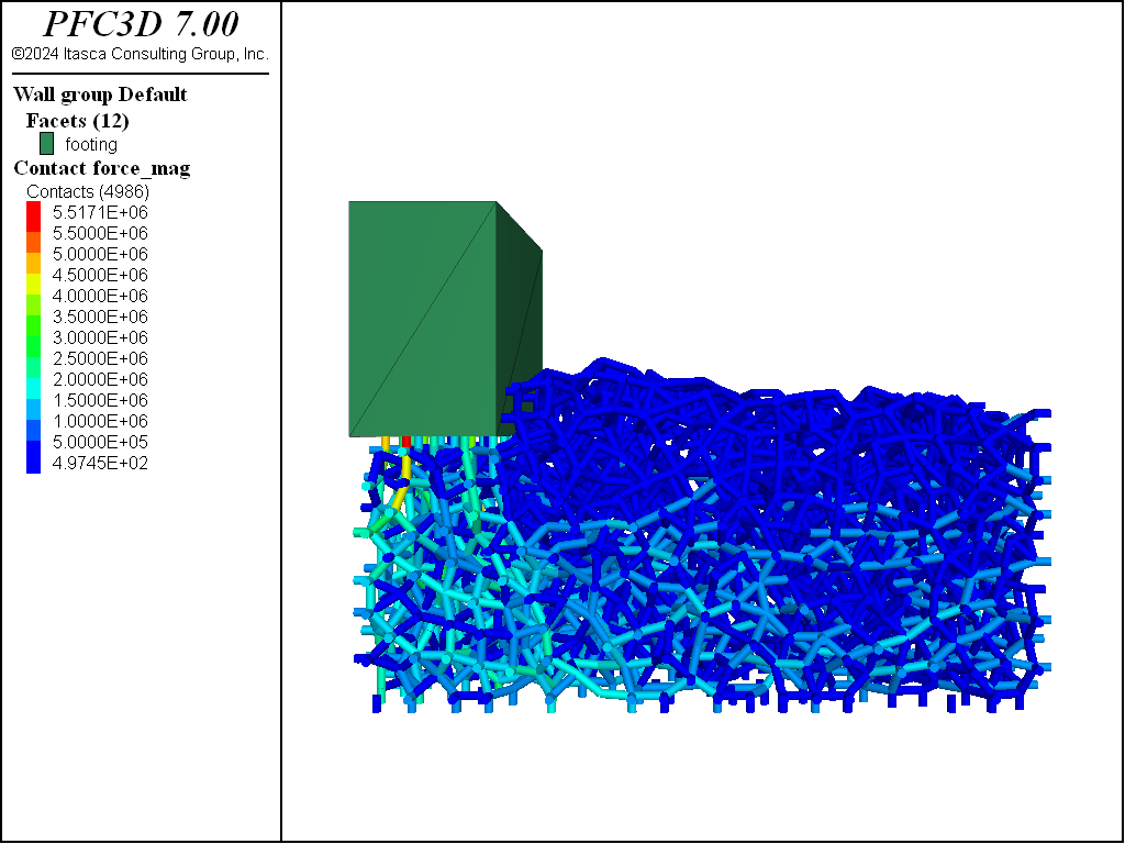
Figure 2: Applied forces resulting from zone face apply stress-normal.
Applied Stress Gradients
The zone face apply command may take the optional keyword gradient, which allows
the applied stresses or forces to vary linearly over the specified range. The parameter
following gradient, v, specifies the \(x\)-, \(y\)-, and \(z\)-variation, respectively,
for the stress- or force-component. The value varies linearly with distance from the global
coordinate origin at (\(x\) = 0, \(y\) = 0, \(z\) = 0):
in which \(S^{(o)}\) is the value at the global coordinate origin at (\(x\) = 0, \(y\) = 0, \(z\) = 0), and \(g_x\), \(g_y\), and \(g_z\) specify the variation of the value in the \(x\)-, \(y\)-, and \(z\)-directions.
The operation of this feature is best explained by an example:
zone face apply stress-xx -10e6 gradient (0,0,1e5) range position-z -100 0
The equation for the \(z\)-variation in stress-component \(\sigma_{xx}\) is
The \(\sigma_{xx}\)-stress at the origin (\(x\) = 0, \(y\) = 0, \(z\) = 0) is \(\sigma_{xx}\) = -10 × 106; at \(z\) = -100, it is -20 × 106. At points in between, the stress is linearly scaled to the relative \(z\)-distance from the origin.
Another option is to use the vary keyword, which may be more familiar from FLAC. See Value Modifiers (add, multiply, gradient, & vary keywords) for further discussion of both options.
Typically, applied stress gradients are used to reproduce the effects of increasing stress with
depth caused by gravity. It is important to make sure that the applied gradient is compatible
with the stress gradient specified with the zone initialize-stresses command. See
Initial Conditions for further comments on stress gradients.
Changing Boundary Stress
It may be necessary to alter the values of applied stresses during the course of a FLAC3D
simulation. For example, the load on a footing may change. To effect a sudden change in an
existing applied stress or load, a new zone face apply command is given, with the range
and stress component given exactly as in the original command, but with a changed value or
variation. In this case, FLAC3D will detect a conflict in the apply condition already present
and remove it. New values will replace existing values for any overlapping
zone face apply commands. It may be necessary to first remove boundary conditions (with
zone face apply-remove) before updating a boundary stress.
In many instances, it may be necessary to change a boundary stress gradually. This is often
required to minimize the shock to a sensitive system, especially if “path-dependence” of the
solution is important (see Localization, Physical Instability and Path-Dependence). The zone face apply command includes options to make gradual application (or removal) of boundary conditions simple and straightforward. For example, to increase the applied stress incrementally while maintaining quasi-equilibrium, you can use the ramp option to the servo keyword:
zone face apply stress-xx -1e5 servo ramp range group 'East' position-z 0,2
Apply changing stress boundary with a FISH function
The servo keyword and its various options is only one way to change the value of an applied boundary over time. Either FISH or tables can be used to add a multiplier to the value. Each step, the table is queried or the FISH function is called, and the value of the applied boundary will be multiplied by the return. A return of 1.0 will therefore have no effect, and a return value of 0.0 will effectively remove the boundary (in the case of stress boundaries). The following is a simple example of using a short FISH function to vary the stress applied sinusoidally.
fish define apply
    apply = math.sin(dynamic.time.total*10)
end
zone face apply stress-xx -1e5 fish apply range group 'East' position-z 0,2
Apply changing stress boundary with table data
The following example creates a simple table that is used to gradually ramp the stress boundary up from nothing. Note that for a table multiplier, you must specify the time value to use as the \(x\) lookup. In this case, we specify dynamic time. By default, a table multiplier will use the current total step number as the \(x\) lookup value.
table 'ramp' add (0,0) (1,1)
zone face apply stress-xx -1e5 table 'ramp' time dynamic ...
                range group 'East' position-z 0,2
Gradual excavation of a circular tunnel
Because FLAC3D uses physics to inform the path it takes to static convergence, sudden changes
to the model can have quasi-inertial effects that may artificially exaggerate damage in the
area. One way to mitigate this is to gradually excavate regions, so that the effect of zone
removal is less sudden. The zone relax excavate command was created for this purpose.
This command is a zone-based apply condition that gradually reduces the stress, stiffness, and
density of the zones in the range until they have effect on the model and are then set to the
null constitutive model. Previous sentence is missing a word, should there be a “no” in
front of “effect?
By default, zone relax uses a servo to automatically maintain quasi-equilibrium, however
the command has any number of options for controlling the exact method of reducing the influence
of zones tagged for excavation.
The following example creates a simple circular tunnel. This tunnel is both excavated instantly
and gradually via zone relax excavate.
model new
model large-strain off
; Create zones
zone create radial-cylinder point 0 0 0 0 point 1 add 18 0 0 ...
                            point 2 add 0 8 0 point 3 add 0 0 18 ...
                            dim 1.75 1.75 1.75 1.75 ratio 1.0 .83 1.0 1.2 ...
                            size 6 6 6 15 fill group 'exc'
zone create radial-cylinder point 0 0 8 0 point 1 add 18 0 0 ...
                            point 2 add 0 8 0 point 3 add 0 0 18 ...
                            dim 1.75 1.75 1.75 1.75 ratio 1.0 1.2 1.0 1.2 ...
                            size 6 6 6 15 fill
zone face skin
; Assign constitutive models and properties
zone cmodel assign mohr-coulomb
zone property bulk 33.33e9 she 25e9 fric 45 cohesion 15e6 ten 5e6
; Assign Boundary Conditions
zone face apply velocity-normal 0 range group 'West' or 'East'
zone face apply velocity-normal 0 range group 'South' or 'North'
zone face apply velocity-normal 0 range group 'Bottom' or 'Top'
; Initial Conditions
zone initialize stress xx -65e6 yy -65e6 zz -65e6
model solve
model save 'initial'
; instantaneous excavation
zone delete range group 'exc'
model solve
model save 'instant'
; gradual excavation
model restore 'initial'
zone relax excavate range group 'exc'
model solve
model save 'relax'
Note that the total number of steps taken to reach equilibrium is actually a little lower when relaxation is used. This is not uncommon.
An examination of the state flags for the zones surrounding the excavation shows that the relaxed version not only shows less damage, but is entirely lacking in tensile failure indicators.
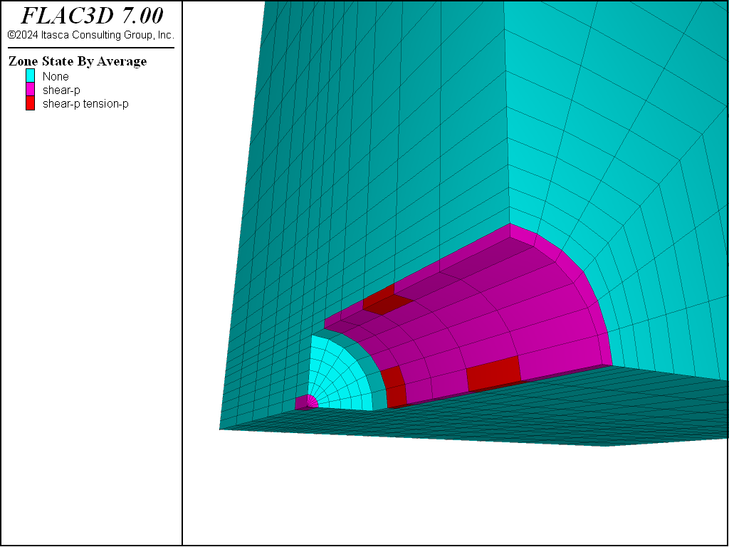
Figure 3: Plasticity state for instantaneous excavation of tunnel.
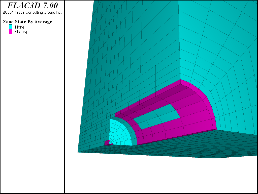
Figure 4: Plasticity state for relaxed excavation of tunnel.
Cautions and Advice
In this section, some miscellaneous difficulties with stress boundaries are described.
With FLAC3D, it is possible to apply stresses to the boundary of a body that has no displacement constraints (unlike many finite-element programs, which require some constraints). The body will react in exactly the same way as a real body would (i.e., if the boundary stresses are not in equilibrium, then the whole body will start moving). The following data file illustrates the effect.
Spin when grid is not in equilibrium
model new
model large-strain off
zone create brick size 6,6,6 point 1 (6,0,-1)
zone cmodel assign elastic
zone property bulk 8e9 shear 5e9
zone face apply stress-xx -2e6 range position-x 0
zone face apply stress-xx -2e6 range position-x 6
model step 500
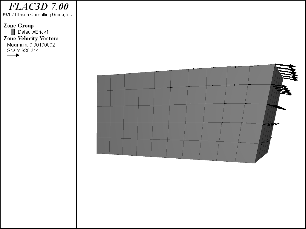
The plots produced from this example are given in the following figure. The applied \(\sigma_{xx}\) stress causes horizontal forces to act on the body. Because the body is tilted, these forces give rise to a moment that causes the body to spin.
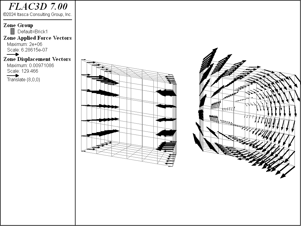
Figure 5: Applied horizontal forces and rotational displacement induced on tilted body.
A similar, but more subtle, effect arises when material is excavated from a body that is supported by a stress boundary condition: the body is initially in equilibrium under gravity, but the removal of material reduces the weight. The whole body then starts moving upward, as demonstrated by the following data file.
Uplift when material is removed
model new
model large-strain off
; Create zones
zone create brick size 5,5,5
zone face skin
; Assign model and properties
zone cmodel assign elastic
zone property bulk 8e9 shear 5e9 density 1000
; Boundary Conditions
zone face apply velocity-normal 0 range group 'West' or 'East'
zone face apply velocity-normal 0 range group 'North' or 'South'
zone face apply stress-normal -5e4 range group 'Bottom'
; Initial Conditions
model gravity 10
zone initialize-stresses
model solve ; Starts at equilibrium
zone cmodel assign null range position (1,1,3) (4,4,5)
model step 100 ; body no longer in equilibrium
The uplift is shown in the next figure. The difficulty encountered in running this data file can be eliminated by fixing the bottom boundary, rather than supporting it with stresses. The Artificial Boundaries section contains some information relating to the location of such artificial boundaries.

Figure 6: Uplift of model when material is removed.
Displacement Boundary
Displacements cannot be controlled directly in FLAC3D; in fact, they play no part in the
calculation process. In order to apply a given displacement to a boundary, it is necessary to
prescribe the boundary’s velocity for a given number of steps. If the desired displacement is
\(D\), a velocity \(V\) over \(N\) steps (where \(N = D/V\)) may be applied. In
practice, \(V\) should be kept small and \(N\) large, in order to minimize shocks to the
system being modeled. The zone face apply command or the zone gridpoint fix and
zone gridpoint initialize commands can be used to specify the velocities; gradients may
also be specified.
Local System and Applied Velocities
Applied velocity conditions always refer to gridpoints, though they may be applied via zone-face
commands (e.g., zone face apply velocity-local) or zone-gridpoint commands. When
zone-face commands are used, all gridpoints connected to selected faces are selected.
Velocities can be applied in terms of the \(x\),\(y\),\(z\)-global axes (i.e., with keywords velocity-x, velocity-y, or velocity-z) or in terms of a local axes (with keywords velocity-dip, velocity-strike, or velocity-normal). All local or global velocity components may be supplied as a vector in one command (with velocity-local v, or velocity v, respectively). The local axes are defined by the normal vector at each gridpoint, using the convention in the figure below:
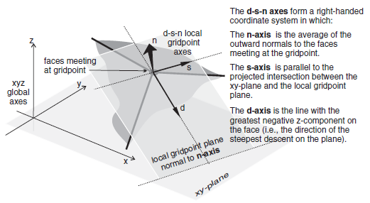
Figure 7: Local gridpoint axes defined by (d) dip direction, (s) strike direction, and (n) normal direction.
Each gridpoint has its own local coordinate system, which can be specified with the
zone gridpoint system command. The zone face apply logic will over-write those
values if necessary to apply the conditions requested. It will also automatically attempt to
rotate and select appropriate local degrees-of-freedom to allow multiple velocity constraints to
be present in the same gridpoint. If this is not possible, then a previous apply condition will
be removed to make way for the new one. This means that it is not necessary to work out a
compatible local system on sloped or irregular boundaries ahead of time. For example, it is
possible to apply roller boundaries to a wedge-shaped block in a single command:
model new
zone create wedge
zone face skin
zone face apply velocity-normal 0 range group 'East'
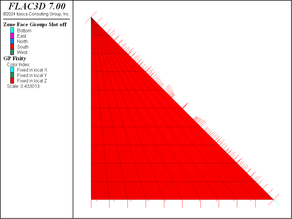
Figure 8: Gridpoint constraints on a wedge-shaped section.
Note that the normal direction was automatically selected on the sloped surface and multiple constraints on the toe were applied. The out of plane degree of freedom in the toe is still free.
Surface Corners and Velocity Boundaries
The gridpoint normal direction used is the average of the normal vectors of the faces included in that apply condition that meet at a gridpoint. This means that care must be taken to select faces that result in the desired normal vector, and commonly, multiple apply commands are necessary to prescribe multiple conditions on gridpoints along boundaries. For example, if one attempted to apply roller boundaries to five sides of a mode in one command with:
zone face apply velocity-normal 0 ...
                range group 'North' or 'South' or 'East' or 'West' or 'Bottom'
then the result can be seen in the following plot of gridpoint fixity. The corners of the model have been fixed at a diagonal, because that is the normal vector calculated using the average of all faces included in that apply that is connected to a gridpoint.
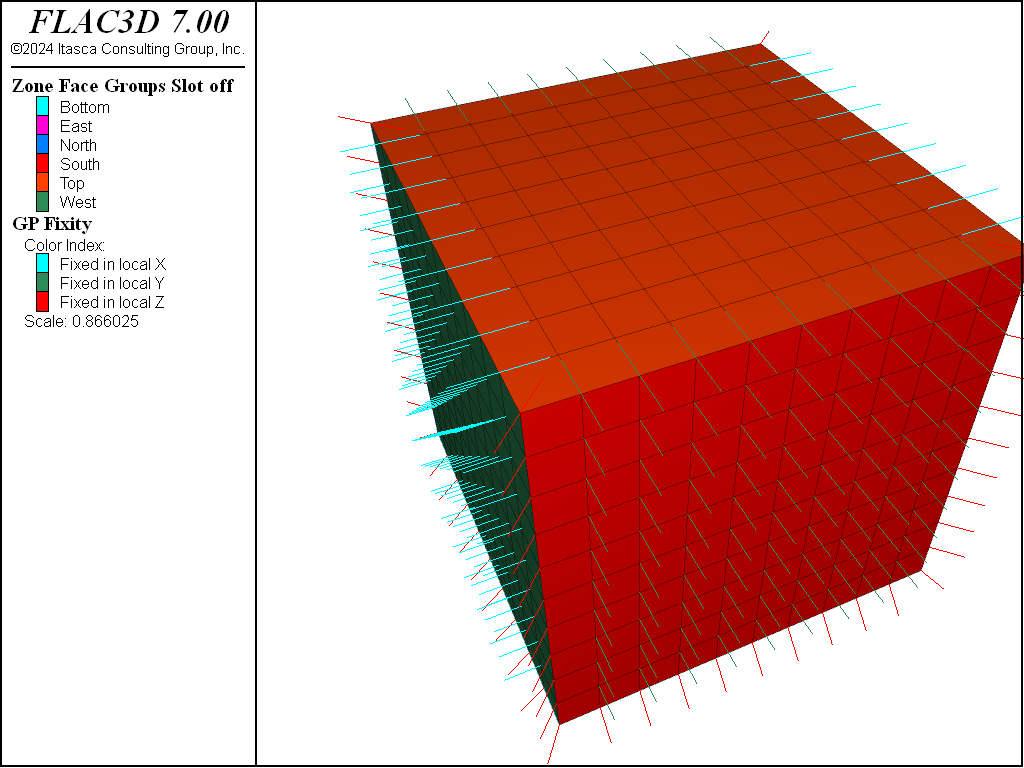
Figure 9: Velocity constraint directions from attempting to apply roller boundaries in a single command.
If the command were split into three, with the ‘East’ and ‘West’ done separately from the ‘North’ and ‘South’ and the ‘Bottom’, then the result is:
zone face apply velocity-normal 0 range group 'West' or 'East'
zone face apply velocity-normal 0 range group 'North' or 'South'
zone face apply velocity-normal 0 range group 'Bottom'
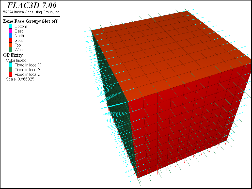
Figure 10: Velocity constraint directions when multiple apply commands are used.
This pattern is seen often in example problems in the FLAC3D documentation. Note that it is acceptable to combine ‘West’ and ‘East’ into one command because those surfaces do not share a boundary.
Velocity conditions can be applied at any orientation by using the local axes. A normal gridpoint direction can be specified arbitrarily for the local axes by using the system keyword; this will override the default normal direction.
Fix vs Apply
Another method of specifying velocities at gridpoints is to use the zone gridpoint fix
command. For example, the following commands are equivalent. Both commands apply a fixed
velocity of (1e-5,0,0) to all gridpoints connected to faces of group East.
zone gridpoint fix velocity (1e-5,0,0) range group 'East'
zone face apply velocity (1e-5,0,0) range group 'East'
In general, using the zone face apply command is preferred because the apply logic uses
the gridpoint local systems and fixity flags. Any values set there manually may be over-ridden
by a later apply condition. Also, the apply logic calculates local systems and attempts to
moderate between multiple constraints automatically. Note, however, that zone face apply
can currently only be performed on surface faces, where zone gridpoint fix can be done on
any gridpoints in the model.
Reaction Forces
When gridpoints are moved rigidly, the reaction forces at the gridpoints can be monitored using FISH. The sum of the reaction forces along a boundary may be obtained with a simple FISH function that adds up the values returned from the gp.force.unbal intrinsic over the desired range. (See Tutorial: Working with FISH.)
Nonuniform Velocities
If nonuniform prescribed velocities are required, the gradient keyword may be used. For a more complicated velocity profile, or one that changes as the simulation proceeds, it will be necessary to write a FISH function. The next example demonstrates this for the model of a rotating retaining wall on the right-hand side of a block of soil.
Rotating retaining wall
model new
; Create zones
zone create brick size 10 5 5
zone face skin
; Constitutive model and properties
zone cmodel elastic
zone property shear 1e8 bulk 2e8
; FISH function
fish operator apply(gp,dum,rate)
    local p = gp.pos(gp)
    local x =  rate * p->z / 5.0
    local z = -rate * (p->x - 10.0) / 5.0
    return vector(x,0,z)
end
; Boundary conditions
zone face apply velocity (0,0,0) range group 'West' or 'Bottom'
zone face apply velocity (1,1,1) fish-local apply(0,0,1e-3) range group 'East'
; Setup
model large-strain on
; Cycle
model step 1000
In this example, the fish-local keyword is used to adjust the velocities at every gridpoint during cycling. The FISH funcion apply is called once for each gridpoint each cycle. The first argument gp is the pointer to the gridpoint. In this case, the second argument is unused. The location of the gridpoint is used to calculate a velocity that in large strain, will cause the right-hand boundary to rotate. The velocity profile of the wall is adjusted as the geometry changes in large-strain mode. Note that the given velocity in this example is much too high for a realistic simulation; it is for demonstration purposes only.
Real Boundaries — Choosing the Right Type
It is sometimes difficult to know which type of boundary condition to apply to a particular surface of the body being modeled. For example, in modeling a laboratory triaxial test, should the load applied by the platen be regarded as a stress boundary, or should the platen be treated as a rigid displacement boundary? Of course, the whole testing machine, including the platen, could be modeled, but that might be very time-consuming. (Remember that FLAC3D takes a long time to converge if there is a large contrast in stiffnesses.) In general, if the object applying the load is very stiff compared with the sample (say, more than 20 times stiffer), then it may be treated as a rigid boundary. If it is soft compared with the sample (say, 20 times softer), then it may be modeled as a stress-controlled boundary. Clearly, a fluid pressure acting on the surface of a body is of the latter category. Footings on soil can often be represented as rigid boundaries that move with constant velocity for the purpose of finding the collapse load of the soil. This approach has another advantage—it is much easier to control the test and obtain a good load/displacement graph. It is well-known that stiff testing machines are more stable than soft testing machines.
Artificial Boundaries
Artificial boundaries fall into two categories: planes of symmetry and planes of truncation.
Symmetry Planes
Sometimes it is possible to take advantage of the fact that the geometry and loading in a system
are symmetrical about one or more planes. For example, if everything is symmetrical about a
vertical plane, then the horizontal displacements on that plane will be zero. Therefore, we can
make that plane a boundary and fix all gridpoints in the horizontal direction using the
zone face apply velocity-normal 0 command, with the range given as the boundary
plane. In the case considered, the \(y\)- and \(z\)-components of velocity on the vertical plane of
symmetry are not affected and should not be fixed. Similar considerations apply to other planes
of symmetry. Planes of symmetry can also be set along boundaries that lie at angles to the \(x\),\(y\),\(z\)-coordinate axes.
Boundary Truncation
When modeling infinite bodies (e.g., tunnels underground) or very large bodies, it may not be possible to cover the whole body with zones, due to constraints on memory and computer time. Artificial boundaries are placed sufficiently far away from the area of interest that the behavior in that area is not greatly affected. It helps to know how far away to place these boundaries, and what errors might be expected in the stresses and displacements computed for the area of interest.
Several points should be considered when selecting the location for artificial boundaries:
- A fixed boundary causes both stresses and displacements to be underestimated, while a stress boundary does the opposite.
- The two types of boundary condition “bracket” the true solution, so that it is possible to do two tests with small boundaries and get a reasonable estimate of the true solution by averaging the two results.
- The effect of boundary location is most noticeable for elastic bodies because the displacements and stress changes are more confined when plastic behavior is present; there is a natural cut-off distance within which most of the action occurs. The artificial boundary may be placed slightly closer without serious error. However, any artificial boundary must not be sufficiently close that it attracts plastic flow and thereby invalidates the solution.
It is always best to run several (coarse) models first, with different boundary locations, to evaluate the potential influence of the boundary on the calculated response, before performing the detailed analysis.
| Was this helpful? ... | 3DEC © 2019, Itasca | Updated: Feb 25, 2024 |