Examples • Example Applications

Undrained Cylindrical Cavity Expansion in a Cam-Clay Medium

Problem Statement

Note

The project file for this example is available to be viewed/run in FLAC3D.[1] The project’s main data file is shown at the end of this example.

The stress and pore-pressure changes due to the expansion of a pressuremeter in a saturated clay mass are analyzed using the model of a cylindrical cavity in an infinite Cam-clay medium. The effect of the finite length of the measuring device is not considered.

In the experiment, the radius \(a\) of the cavity is expanded up to twice its original size, \(a_0\). The properties of the Cam-clay material, which correspond to a Boston Blue Clay, are as follows (Carter et al. 1979):

undrained cohesion (\(C_u\))	1 MPa
shear modulus (\(G\))	74 × \(C_u\)
soil constant (\(M\))	1.2
slope of normal consolidation line (λ)	0.15
slope of elastic swelling line (κ)	0.03
reference pressure (\(p_1\))	\(C_u\)
specific volume at reference pressure (\(v_λ\))	2.3

The clay is normally consolidated with in-situ stresses \(σ'_r\) = \(σ'_θ\) = -1.65 \(C_u\), \(σ'_z\) = -3 \(C_u\) and initial excess pore pressure \(u_e\) = 0. The shear modulus of the material is assumed to remain constant during the simulation. The pressuremeter membrane is considered impermeable, and the fluid bulk modulus is much larger than that of the soil so that the numerical simulation can be carried out under undrained conditions.

FLAC3D Model

The FLAC3D model is constructed by taking into consideration the axisymmetric and plane-strain properties of the problem. A pie slice corresponding to one-tenth of a quadrant and of height \(h\) is considered (see the front view in Figure 1). The FLAC3D model is of finite extent, but the length \(L\) is chosen as very large compared to \(a_0\).

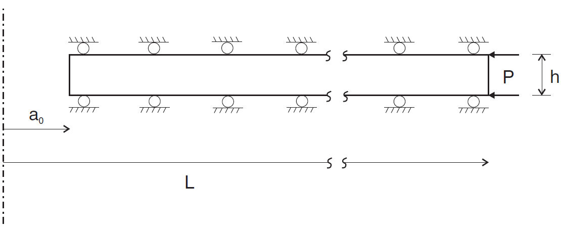
Figure 1: Front view of the model geometry.

The dimensions of the FLAC3D grid correspond to dimensionless values \(a_0\)/\(a_0\) = 1, \(L\)/\(a_0\) = 200 and \(h\)/\(a_0\) = 1. The grid is composed of a single layer of 31 zones of constant height and variable zone width, graded by a factor 1.1 (see Figure 2), where the FLAC3D system of reference axes is also represented.

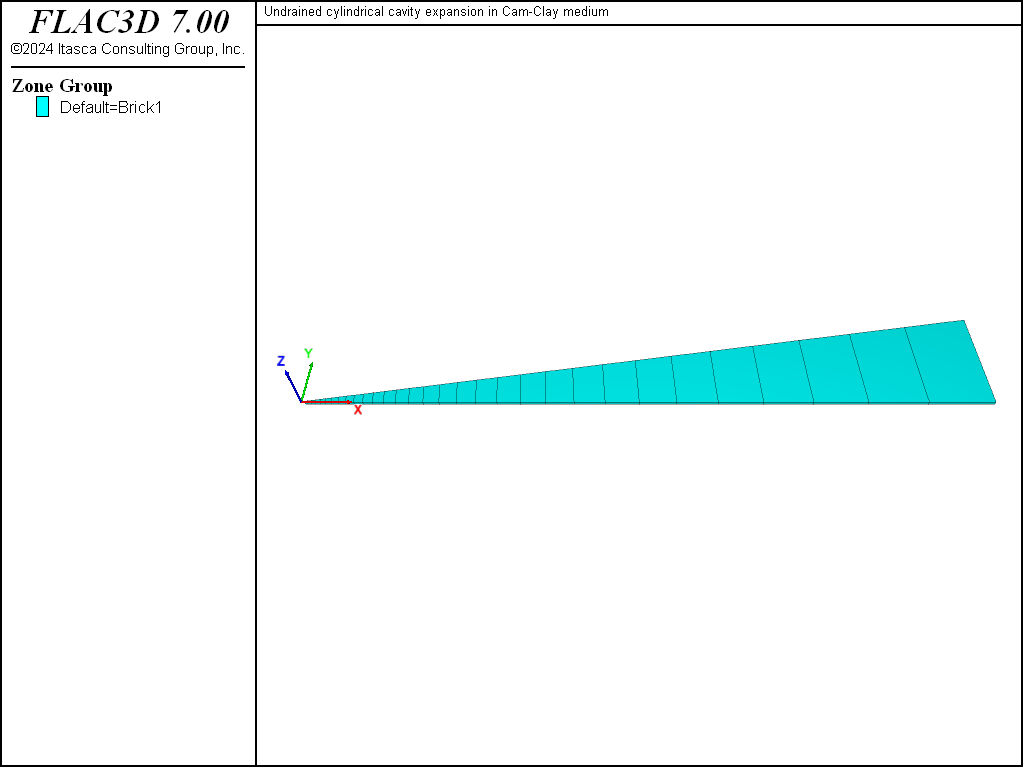
Figure 2: Grid geometry.

Initially, the cavity boundary is fixed, in-situ stresses are installed, and a pressure boundary condition of magnitude 1.65 \(C_u\) is applied at the far \(x\)-boundary. The groundwater configuration (model configure fluid) is selected, and the no-flow (model fluid active off) and large-strain (model large-strain on) options are specified.

The pre-consolidation pressure must be supplied to the numerical model. Since the soil is normally consolidated, this value is calculated from the given initial state. The corresponding values of mean pressure and deviator stress are \(p'_0\) = 2.1 \(C_u\) and \(q_0\) = 1.35 \(C_u\), and the pre-consolidation pressure, evaluated from the Cam-clay yield function (see <section 1 in Constitutive Models>), preceding link waiting to be built for final location of CModel material

(1)\[p'_{c0} = p'_0 [1 + (q_0/(Mp'_0))^2]\]

is 2.70 \(C_u\). For information, the value of the over-consolidation ratio \(R\), defined as \(R\) = \(p^{\prime}_{c0}\)/\(p'_0\), is approximately 1.29 for this problem.

As an illustration, initial values for the specific volume, \(v_0\) , and tangent bulk modulus, \(K_0\) , are specified. They correspond to the default values that would have been assigned by the code at the first step command.

\[v_0 = v_{\lambda} - \lambda \ln (p'_{c0}/p'_1) + \kappa \ln (p'_{c0}/p'_0)\]

\[K_0 = {v_0 p'_0 \over \kappa}\]

By default, the Biot coefficient is equal to one. The Biot modulus (water bulk modulus divided by porosity) is set to 100 times \(K_0\). The maximum bulk modulus is set to 10 times the initial value.

A compressive velocity of magnitude 10^-5 is applied at the cavity boundary for a total of 100,000 steps, so that the cavity radius has doubled at the end of the pressure test. Stresses and pore pressure are monitored during the calculation.

The data file for this problem is listed at the end of this section. The Cam-clay parameters are calculated in the FISH function setProp.

FLAC3D Results and Discussion

The evolution during the expansion of the deviator stress, \(q\)/\(C_u\), at the cavity wall is plotted in Figure 3. The numerical results indicate a failure level at \(q\)/\(C_u\) = 1.777. This value can be compared to the Cam-clay analytical prediction as follows. Under undrained conditions, the yield path followed by a normally consolidated stress point has the form (see the verfication problem Drained and Undrained Triaxial Compression Test on a Cam-Clay Sample).

\[{p'_0\over p'} = {\left({ {M^2+\eta^2}\over{M^2+\eta^2_0} }\right)}^{\Lambda}\]

where \(\eta = q/p'\) and \(\Lambda = (\lambda-\kappa)/\lambda\). The initial value \(\eta_0 = q_0/p'_0\) can be derived from equation (1) above. Using the definition of \(R\), we obtain

\[\eta^2_0 = R M^2 - M^2\]

and the stress path becomes

\[{p'_0\over p'} = {\left({ {M^2+\eta^2}\over{R M^2} }\right)}^{\Lambda}\]

Intersection of this stress path with the critical state line \(q = M p'\) or \(\eta = M\) gives

\[q_{cr} = Mp'_0 \left[{2\over R}\right]^{-\Lambda}\]

The prediction of \(q_{cr}/C_u\) derived from this formula is 1.771, which is in close agreement with that obtained numerically.

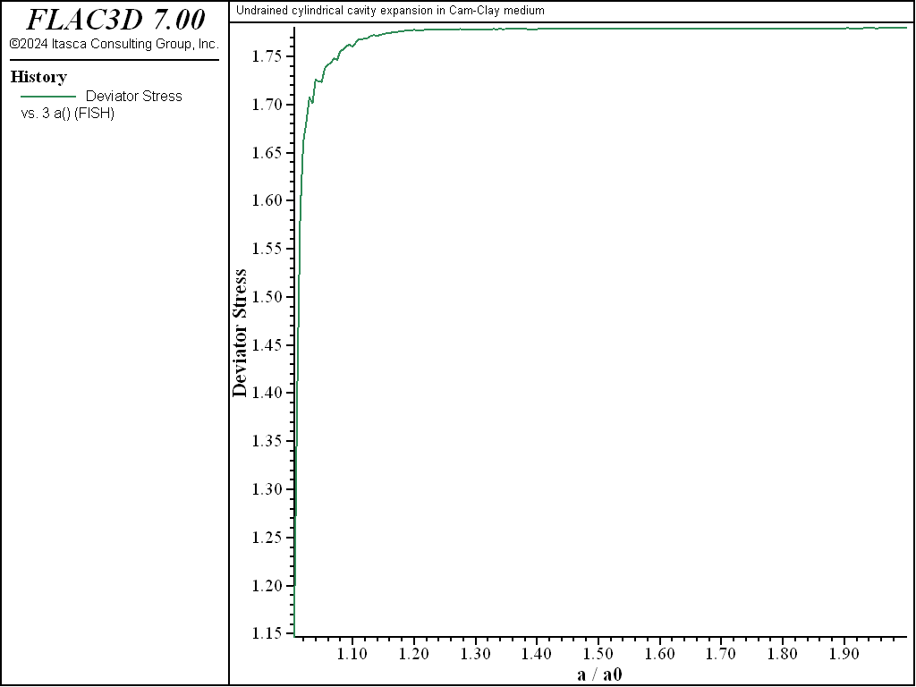
Figure 3: Deviator stress \(q\)/\(C_u\) at the cavity wall versus \(a\)/\(a_0\).

The variation of excess pore pressure and total radial stress at the cavity wall as the cavity expands is illustrated in Figure 4. These curves show a sharp rise followed by a gentle slope as pore pressure and radial stress approach a limit value.

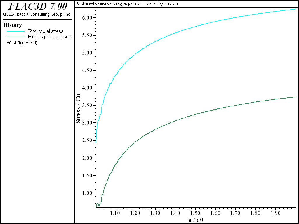
Figure 4: Total radial stress \(σ_r\)/\(C_u\) and excess pore pressure \(u_e\)/\(C_u\) at the cavity wall versus \(a\)/\(a_0\).

The radial distribution of effective stresses and pore pressure when \(a\) = 2 \(a_0\) is plotted in Figure 5. The stresses remain constant in an annulus around the cavity where the soil is at the critical state. There, the distribution of stresses has been greatly affected by the process of cavity expansion, with radial and tangential stresses now in the role of minor and major principal stresses. The excess pore pressure develops mainly in this region. Farther out, the stresses and pore pressure are shown to evolve towards their in-situ values. These results compare well with those presented by Carter et al. (1979).

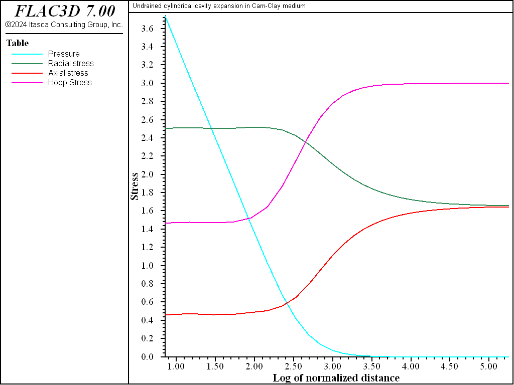
Figure 5: Radial distribution of effective stresses and pore pressure when \(a\) = 2 \(a_0\) plotted versus \(ln\) ( \(r\)/\(a_0\) ) (Table 10 is pore pressure; Tables 11, 12, and 13 are radial, axial, and tangential components of effective stress).

Reference

Carter, J. P., M. F. Randolph and C. P. Wroth. “Stress and Pore Pressure Changes in Clay during and after the Expansion of a Cylindrical Cavity,” International Journal for Numerical and Analytical Methods in Geomechanics, 3, 305-322 (1979).

Data File

CavityExpansion.dat

;-----------------------------------------------------------
; Undrained cylindrical cavity expansion in Cam-Clay medium
;-----------------------------------------------------------
model new
fish automatic-create off
model title "Undrained cylindrical cavity expansion in Cam-Clay medium"
model config fluid
; --- model geometry ---
zone create brick point 0  1.0       0.0       1.0   ...
                  point 1  200.0     0.0       1.0   ...
                  point 2  1.0       0.0       0.0   ...
                  point 4  200.0     0.0       0.0   ...
                  point 3  0.9877    0.1564    1.0   ...
                  point 6  197.5377  31.2869   1.0   ...
                  point 5  0.9877    0.1564    0.0   ...
                  point 7  197.5377  31.2869   0.0   ...
                  size 31 1 1 ratio 1.1 1 1
zone face skin ; Name model boundaries
; --- model properties ---
zone cmodel assign modified-cam-clay
zone property shear 74.
zone property ratio-critical-state 1.2 lambda 0.15 kappa 0.03 ...
              pressure-reference 1.0 specific-volume-reference 2.3
zone initialize stress xx -1.65 yy -1.65 zz -3.
program call 'utility' suppress ; FISH functions used by the example
[effectivePressure]      ; Initializes pressure-effective property
zone fluid cmodel assign isotropic
; --- boundary conditions ---
zone face apply velocity-normal 0   range group 'North'
zone face apply velocity-normal 0   range group 'South'
zone face apply velocity-normal 0   range group 'Top'
zone face apply velocity-normal 0   range group 'Bottom'
zone face apply stress-normal -1.65 range group 'East'
zone gridpoint fix velocity ...
     range group 'West'
zone gridpoint initialize velocity-x  1e-5 ...
     range group 'West' group 'South'
zone gridpoint initialize velocity-y -1e-5 local ...
     range group 'West' group 'North'
; model settings ---
zone fluid biot on
model fluid active off
model large-strain on
; --- histories ---
history interval 500
fish history name='srad' srad
fish history name='p_fl' p_fl
fish history name='a'    a
fish history name='q'    q
; --- test ---
[setProp] ; Initializes biot mod, pressure-preconsolidation, and bulk-maximum
model step 100000
model save 'cavity'

Endnotes

[1]	To view this project in FLAC3D, use the program menu. Help ▼ Examples…   ⮡   FLAC     ⮡   ExampleApplications       ⮡   Expansion         ⮡   CavityExpansion.prj