Examples • Example Applications

Wheel Load over a Buried Pipe

Problem Statement

Note

To view this project in FLAC3D, use the menu command Help ► Examples…. Choose “ExampleApplications/WheelLoadOverBuriedPipe” and select “WheelLoadOverBuriedPipe.prj” to load. The project’s main data file is shown at the end of this example.

A steel pipe is buried at a shallow depth beneath a roadway. An analysis is required to evaluate the effect of wheel loading on the deformation at the road surface, the deflection of the pipe, and stresses within the pipe.

The top of the pipe is 1.4 m beneath the road surface. The pipe has an outer diameter of 4 m and is 0.12 m thick. The pipe excavation is 14 m wide and 5.8 m deep. The pipe is placed on a 0.4 m thick layer of soil backfill, and then soil is compacted around the pipe.

A wheel load is applied above the pipe at a distance of 1.25 m from the \(y\) = 0 plane. The wheel load is applied to four gridpoints on the surface. If the load is assumed to be carried by 1/2 of each zone connected to the gridpoints, then the wheel area can be assumed to be 1.275 m². The wheel load is increased until failure occurs in the soil. The analysis determines the failure load and the resulting soil settlement, pipe displacement, and stresses.

Modeling Procedure

The FLAC3D model assumes symmetric conditions about a vertical plane through the center of the pipe and a vertical plane midway between the wheel loads. The model grid is shown in Figure 1. The \(x\) = 0 plane corresponds to the vertical plane through the center of the pipe, and the \(y\) = 0 plane corresponds to the plane midway between wheel loads. The model contains 1344 zones, with finer zoning in the vicinity of the applied wheel load.

For these model conditions, it is assumed that, if the pipe buckles, this will occur in the circular plane of the pipe. Buckling along the pipe is considered unlikely and is excluded in the analysis. A full model of the pipe is required if buckling along the pipe is expected.

The soil backfill is represented as a Mohr-Coulomb material with several properties listed in Table 1:

Table 1: Soil Properties

density	2000 kg/m3
shear modulus	0.30 × 108 Pa
bulk modulus	0.65 × 108 Pa
friction angle	34°
dilation angle	20°
cohesion	5.0 × 103 Pa
tensile strength	103 Pa

The wheel load is simulated by applying a constant velocity to the gridpoints within the wheel load area. A \(z\)-direction velocity of -2.5 × 10^-5 m/step is applied for 6000 steps. The wheel-bearing pressure is monitored during loading with a FISH function, wload.

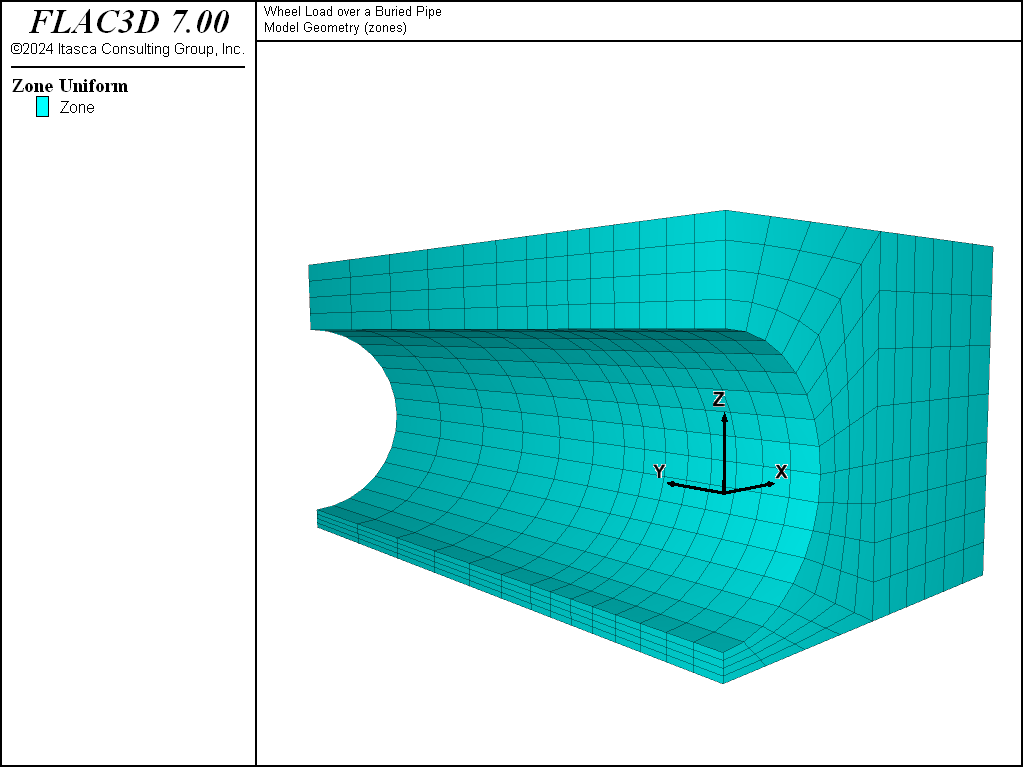
Figure 1: Shallow pipe model.

The steel pipe is represented by structural (shell) elements. Figure 2 shows the shell element geometry. The pipe consists of 448 structural elements and 255 structural nodes. The Young’s modulus of the steel is 227 GPa and the Poisson’s ratio is 0.25.

This analysis is performed in large-strain mode to provide a clearer representation of the settlement profile of the soil. The model is first run to an equilibrium state under gravitational loading; the maximum initial displacement is 1.11 mm at the road surface and 0.92 mm at the crown of the pipe. The displacements are reset to zero, and the \(z\)-velocity is then applied to simulate the wheel load.

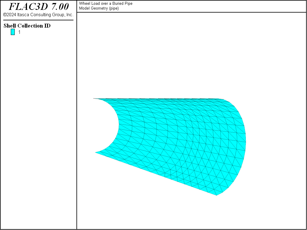
Figure 2: Structural shell (SEL) elements representing pipe.

Results and Discussion

The displacement at the road surface due to the wheel load is 15 cm after 6000 steps. Figure 3 plots the wheel-bearing pressure versus the surface settlement. This plot indicates that the wheel-bearing pressure at which failure of the soil occurs is approximately 400 kPa. The pressure continues to increase as a result of the support provided by the pipe: the pressure reaches 750 kPa after 6000 steps.

The surface settlement is shown by the displacement contour and vector plot in Figure 4. This plot illustrates the region of maximum deflection directly beneath the wheel load. A profile of the grid displacement along the axis of the pipe is shown in Figure 5, and a profile normal to the pipe axis is shown in Figure 6.

The histories of vertical displacement at the road surface beneath the wheel load and at the top of the pipe are plotted in Figure 7. At 15 cm surface displacement, the top of the pipe has deflected 2.6 cm. Figure 8 plots contours of displacement within the shell elements. Note that these are total displacements (including displacement due to gravity).

The distribution in stress at the interior pipe surface is shown by the contour plot of minimum (i.e., major) principal stress in Figure 9. The FISH function mises calculates the maximum von Mises stress invariant in the pipe. The maximum von Mises stress is at the inner pipe surface and is calculated to be approximately 200,000 kPa.

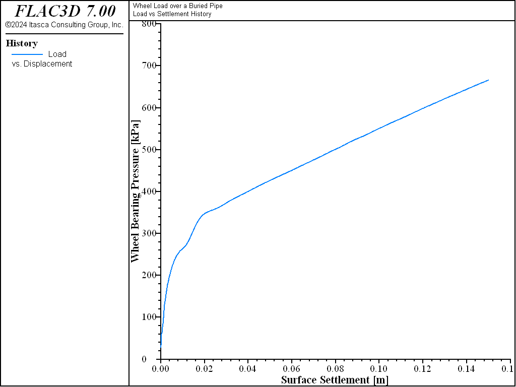
Figure 3: Wheel-bearing pressure (kPa) versus surface settlement (m).

Figure 4: Displacement (m) resulting from the wheel load.

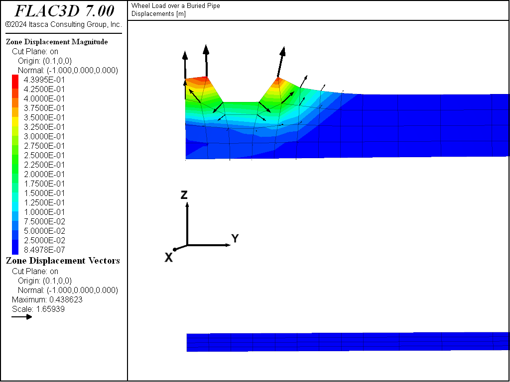
Figure 5: Displacement (m) on a vertical plane along the pipe axis.

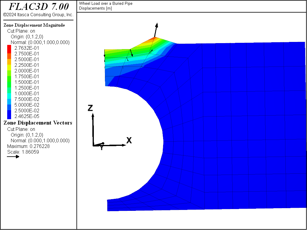
Figure 6: Displacement (m) on a vertical plane normal to the pipe axis.

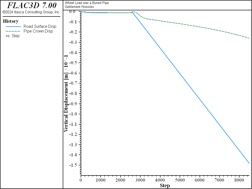
Figure 7: History of vertical displacement (m) at the road surface (solid line) and at the pipe crown (dashed line) beneath the wheel load.

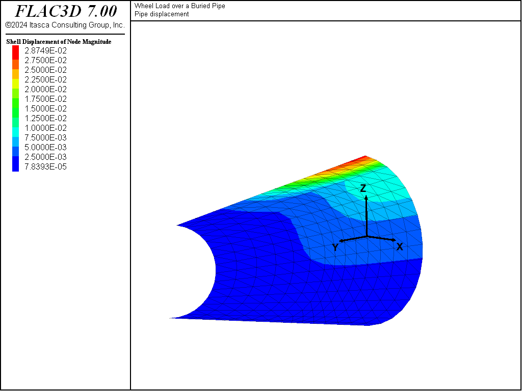
Figure 8: Contours of deflections (m) in the pipe resulting from gravitational loading and the wheel load.

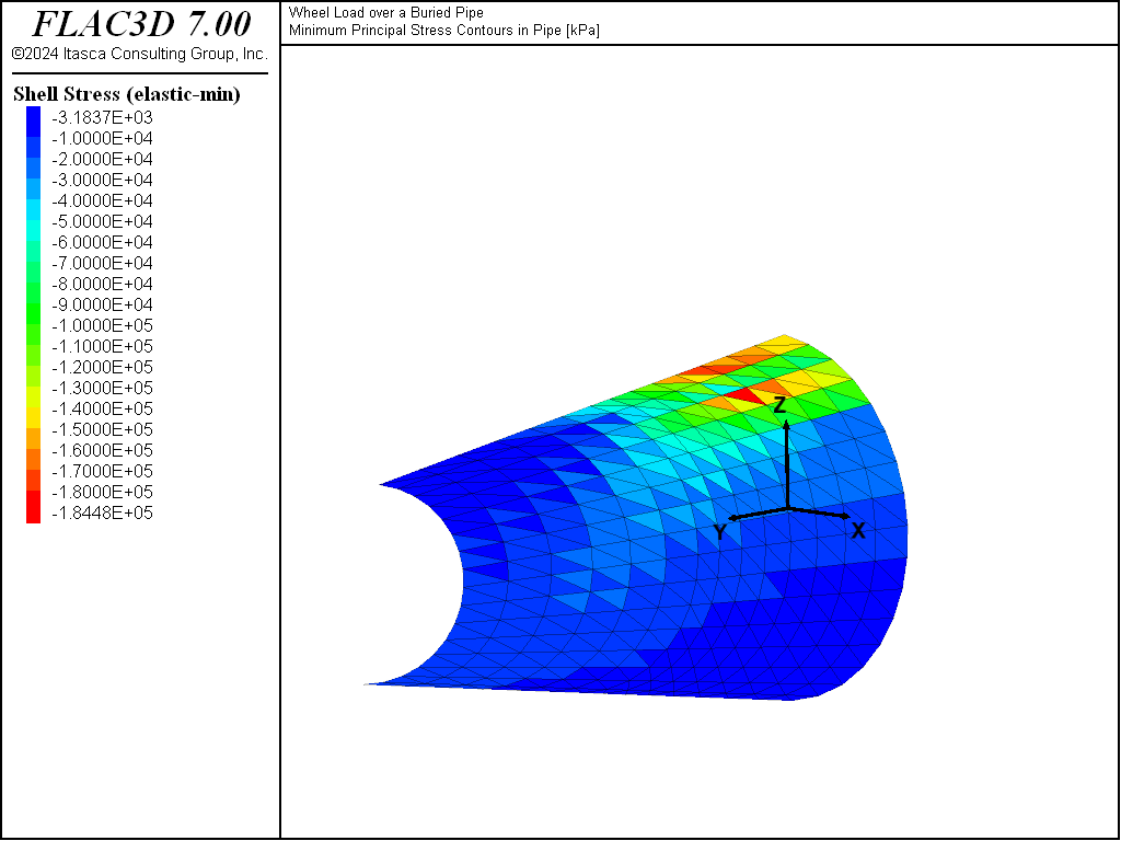
Figure 9: Contours of minimum principal stress (kPa) in pipe resulting from gravitational loading and wheel load.

Data File

WheelLoadOverBuriedPipe.dat

; ==================================================================
;   FLAC3D analysis of a wheel load over a buried pipe
; ==================================================================
model new
fish automatic-create off
model title 'Wheel Load over a Buried Pipe'
;  generate geometry from extruder tool, saved from State Record
program call 'geometry' suppress
zone generate from-extruder
zone face skin ; Label model boundaries
; Tag the face to be loaded
zone face group 'loadedFace' range position-x -0.1 0.9 ...
                position-y 0.9 1.6  position-z 3.3 3.6
;  assign Mohr-Coulomb model to soil (stress units: kPa)
zone cmodel assign mohr-coulomb
model gravity 10
zone property bulk 65000 shear 30000 density 2.0
zone property cohesion 5.0 friction 34 tension 1.0 dilation 20
;
model large-strain on
; Apply roller boundaries
zone face apply velocity-normal 0 range group 'Bottom1'
zone face apply velocity-normal 0 range group 'East' or 'West2' or 'West1'
zone face apply velocity-normal 0 range group 'North' or 'South'
;
zone history name 'zwheel' displacement-z position (0,1,3.4)
zone history name 'zpipe'  displacement-z position (0,1,2)
model save 'geometry'
;  add pipe
struct shell create by-zone-face range group 'pipeFace' ; Group assigned 
                                                   ; in extruder.
struct shell property isotropic 227e6 0.25  thickness 0.012
; Boundary conditions for shell
struct node fix velocity-y rotation-x rotation-z range position-y 0
struct node fix velocity-y rotation-x rotation-z range position-y 12
struct node fix velocity-x rotation-y rotation-z range position-x 0
; Solve for initial gravity loading.
model solve ratio-local 1e-4
model save 'initial'
; Reset displacements
zone gridpoint initialize displacement (0,0,0)
; Apply wheel load at surface
zone face apply velocity-z -2.5e-5 range group 'loadedFace'
; Calculate applied load
[global gplist = gp.list(gp.isgroup(::gp.list, 'loadedFace'))]
fish define load
    return list.sum(gp.force.unbal.z(::gplist)) / 1.275
end
fish history name 'load' load
model step 6000 ; 0.15 total displacement on wheel
; stress recovery ...
struct shell recover surface (1,2,3)
struct shell recover stress depth-factor 1.0
program call 'mises' suppress ; FISH function to find maximum von-mises stress
fish list [mises]
; Save the final state
model save 'load'