Mohr-Coulomb Model
The failure envelope for this model corresponds to a Mohr-Coulomb criterion (shear yield function) with tension cutoff (tension yield function). The position of a stress point on this envelope is controlled by a nonassociated flow rule for shear failure, and an associated rule for tension failure.
Formulations
The Mohr-Coulomb criterion in FLAC3D or 3DEC is expressed in terms of the principal stresses
\({\sigma}_1, {\sigma}_2\), and \({\sigma}_3\), which are the three components of the generalized stress vector for this model (\(n\) = 3). The components of the corresponding generalized strain vector are the principal strains \({\epsilon}_1, {\epsilon}_2\), and \({\epsilon}_3\).
Incremental Elastic Law
The incremental expression of Hooke’s law in terms of the generalized stress and stress increments has the form
where \({\alpha}_1\) and \({\alpha}_2\) are material constants defined in terms of the shear modulus, \(G\), and bulk modulus, \(K\), as
For future reference, comparing those expressions on \(S_i\) in Incremental Formula:
Composite Failure Criterion and Flow Rule
The failure criterion used in the model is a composite Mohr-Coulomb criterion with tension cutoff. In labeling the three principal stresses so that
this criterion may be represented in the plane \(({\sigma}_1,{\sigma}_3)\) as illustrated in Figure 1. (Recall that compressive stresses are negative.) The failure envelope \(f({\sigma}_1,{\sigma}_3)\) = 0 is defined from point \(A\) to \(B\) by the Mohr-Coulomb failure criterion \(f^s\) = 0 with
and from \(B\) to \(C\) by a tension failure criterion of the form \(f^t\) = 0 with
where \(\phi\) is the friction angle, \(c\) is the cohesion, \({\sigma}^t\) is the tensile strength, and
Note that the tensile strength of the material cannot exceed the value of \({\sigma}_3\) corresponding to the intersection point of the straight lines \(f^s\) = 0 and \({\sigma}_1 = {\sigma}_3\) in the \(f({\sigma}_1,{\sigma}_3)\) plane. This maximum value is given by
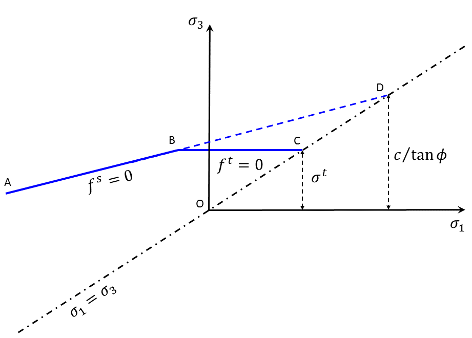
Figure 1: FLAC3D Mohr-Coulomb failure criterion.
The potential function is described by means of two functions, \(g^s\) and \(g^t\), used to define shear plastic flow and tensile plastic flow, respectively. The function \(g^s\) corresponds to a nonassociated law and has the form
where \(\psi\) is the dilation angle and
The function \(g^t\) corresponds to an associated flow rule and is written
The flow rule is given a unique definition by application of the following technique. A line represented by the diagonal between the representation of \(f^s\) = 0 and \(f^t\) = 0 in the \(({\sigma}_1, {\sigma}_3)\)-plane (see Figure 2) divides the domain where an elastic guess violating the composite yield function into two domain: domain 1 and domain 2 (see Figure 2).
If the stress point falls within domain 1, shear failure is declared and the stress point is placed on the curve \(f^s\) = 0 using a flow rule derived using the potential function \(g^s\). If the point falls within domain 2, tensile failure takes place, and the new stress point conforms to \(f^t\) = 0 using a flow rule derived using \(g^t\).
Note that by ordering the stresses as in Equation (4), the case of a shear-shear edge is automatically handled by a variation on this technique. The technique, applicable for small-strain increments, is simple to implement: at each step, only one flow rule and corresponding stress correction is involved in case of plastic flow. In particular, when a stress point follows an edge, it receives stress corrections alternating between two criteria. In this process, the two yield criteria are fulfilled to an accuracy which depends on the magnitude of the strain increment. Results obtained for the oedometric test are presented as a validation of this approach.
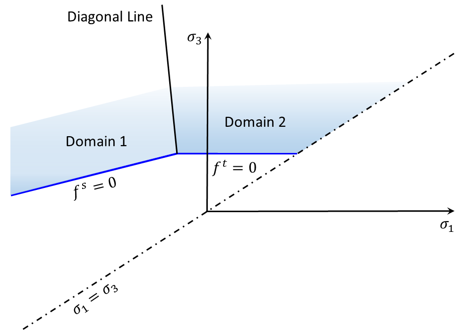
Figure 2: Mohr-Coulomb model—domains used in the definition of the flow rule.
Shear Plastic Corrections
First, considering shear failure, partial differentiation of Equation (9) yields
Substitution of \(\partial g^s / \partial {\sigma}_1\), \(\partial g^s / \partial {\sigma}_2\), and \(\partial g^s / \partial {\sigma}_3\) for \(\Delta {\epsilon}_1^e\), \(\Delta {\epsilon}_2^e\), and \(\Delta {\epsilon}_3^e\), respectively, in Equation (3) gives
Using \(f = f^s\) (see Equation (5))
and
Tension Plastic Corrections
First, we assume the case that there is only one principal stress in tension failure. Partial differentiation of Equation (9) gives
Using Equation (3), we obtain
With \(f = f^t\), as given by Equation (6)
and
Substitution of Equation (15) for \({\lambda}^t\) in Equation (18) gives
After evaluation of \({\sigma}_1^N\), \({\sigma}_2^N\), and \({\sigma}_3^N\), the stress-tensor components are evaluated in the system of reference axes, assuming that the principal directions have not been affected by the occurrence of a plastic correction.
Second, we assume the case that there are two principal stresses in tension failure, or
Partial differentiation of Equation (21) gives
so
From Equation (23) (and remember \(f_y^t(\sigma_2^N) = 0\) and \(f_z^t(\sigma_3^N) = 0\) after plastic correction) we get
Substitution of Equation (24) in Equation (23) gives
Finally, for the case that all three principal stresses are in tension failure, or
similarly,
so
From Equation (28), we get
Remember \(f_x^t(\sigma_2^N) = 0\), \(f_y^t(\sigma_2^N) = 0\) and \(f_z^t(\sigma_3^N) = 0\) after plastic correction, so
Apex Stress Correction
It is possible that one or more corrected principal stresses are greater than the apex stress (\(c/\tan{\phi}\)) at an extreme circumstance when the friction angle is not zero (usually after shear plastic corrections). Once this occurs, all principal stresses will be forced to the apex stress.
Implementation Procedures
In the implementation of the Mohr-Coulomb model in FLAC3D, an elastic guess (\({\sigma}_{ij}^I\)) is first computed by adding to the stress components, increments calculated by application of Hooke’s law to the total strain increments \(\Delta {\epsilon}_{ij}\) (see Elastic Model). Principal stresses \({\sigma}_1^I\), \({\sigma}_2^I\), \({\sigma}_3^I\) and corresponding directions are then calculated.
Following sentence is unclear. What is “it” in second half? If the stresses \({\sigma}_1^I\), \({\sigma}_2^I\), \({\sigma}_3^I\) violate the composite yield criterion (see Equation (5) and (6)), then it is either in domain 1 or domain 2. In the first case, shear failure takes place, and \({\sigma}_1^N\), \({\sigma}_2^N\), and \({\sigma}_3^N\) are evaluated from Equation (14), using Equation (15). In the second case, tensile failure occurs, and new principal stress components are evaluated from from Equation (18) through Equation (30).
If the point \(({\sigma}_1^I, {\sigma}_3^I)\) is located below the representation of the composite failure envelope in the plane \(({\sigma}_1, {\sigma}_3)\), no plastic flow takes place for this step, and the new principal stresses are given by \({\sigma}_i^I\), \(i\) = 1,3.
The stress tensor components in the system of reference axes are then calculated from the principal values by assuming that the principal directions have not been affected by the occurrence of a plastic correction.
The default value for the tensile strength, \(\sigma^t\), is zero. This value is set to \(\sigma_{max}^t\) (see Equation (8)) if the value assigned to the tensile strength exceeds \(\sigma_{max}^t\). By default, if tensile failure occurs in a zone, the value assigned for the tensile strength in this zone remains constant. Alternatively, if the property keyword flag-brittle is set true, then tensile strength is set to zero for that zone when tensile failure occurs. This simulates instantaneous tensile softening.
mohr-coulomb Model Properties
Use the following keywords with the zone property (FLAC3D) or block zone property (3DEC) command to set these properties of the Mohr-Coulomb model.
- mohr-coulomb
- bulk f
elastic bulk modulus, \(K\)
- cohesion f
cohesion, \(c\)
- friction f
internal angle of friction, \(\phi\)
- poisson f
Poisson’s ratio, \(\nu\)
- shear f
elastic shear modulus, \(G\)
- young f
Young’s modulus, \(E\)
- flag-brittle b (a)
If true, the tension limit is set to 0 in the event of tensile failure. The default is false.
Key
- (a) Advanced property.
- This property has a default value; simpler applications of the model do not need to provide a value for it.
- Notes
- Only one of the two options is required to define the elasticity: bulk modulus \(K\) and shear modulus \(G\), or Young’s modulus \(E\) and Poisson’s ratio \(\nu\). When choosing the latter, Young’s modulus \(E\) must be assigned in advance of Poisson’s ratio \(\nu\).
- The tension cut-off is \({\sigma}^t = min({\sigma}^t, c/\tan \phi)\).
| Was this helpful? ... | FLAC3D © 2019, Itasca | Updated: Feb 25, 2024 |