Oedometer Test with Mohr-Coulomb Model
Note
The project file for this example is available to be viewed/run in FLAC3D.[1] The project’s main data file is shown at the end of this example.
This example concerns the determination of stresses in a Mohr-Coulomb material subjected to an oedometer test. In this experiment, two of the principal stress components are equal and, during plastic flow, the stress point evolves along a vertex of the Mohr-Coulomb criterion representation in the \(\Pi\)-plane (the iso-pressure (\(\sigma_{kk}\) = constant) plane in the principal stress space). The purpose is to validate the numerical technique adopted in FLAC3D to handle such a situation. Note that FLAC3D uses no special techniques to deal with yield at vertex points of the Mohr-Coulomb failure locus in the \(\Pi\) plane. Results of a numerical experiment are presented and compared to an exact solution.
The boundary conditions for the oedometric test are sketched in Figure 1. They correspond to the uniform strain rates
where \(v\) is the constant \(y\)-component of the velocity applied to the sample \((v < 0)\), and \(L\) is the height of the sample.
Assuming zero initial stresses, the principal directions of stresses and strains are those of the coordinate axes. For simplicity, we consider a sample of unit height \(L\) = 1.
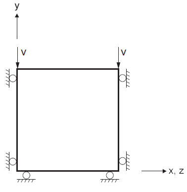
Figure 1: Boundary conditions for oedometer test.
In the elastic range, application of Hooke’s law gives, using \({\epsilon}_{22} = v t\) at time \(t\):
where \(\alpha_1 = K + 4/3 G\) and \(\alpha_2 = K - 2/3 G\).
To apply the Mohr-Coulomb failure criterion, we consider the yield functions
At the onset of yield, \(f^1 = f^2\) = 0 and, using Equations (2) and (3), we find
Hence, yielding will only take place provided \(\alpha_1 - \alpha_2 N_{\phi} >\) 0.
During plastic flow, the strain increments are composed of elastic and plastic parts, and we have
Using the boundary conditions of Equation (1):
The flow rule for plastic flow along the edge of the Mohr-Coulomb criterion corresponding to \({\sigma}_{11} = {\sigma}_{33}\) has the form (e.g., see Drescher 1991)
where \(g^1\) and \(g^2\) are the potential functions corresponding to \(f^1\) and \(f^2\):
After partial differentiation, Equation (7) becomes
In further considering that by symmetry \(\lambda_1 = \lambda_2\), we obtain
The stress increments, derived from Hooke’s law, are given by the relations
where we have used the symmetry condition \(\Delta {\epsilon}_{11}^e = \Delta {\epsilon}_{33}^e\).
Substitution of Equation (6) in Equation (11) yields, using Equation (10):
The parameter \(\lambda_1\) can now be determined by expressing the condition that during plastic flow, \(\Delta f^1\) = 0. Using Equation (3), this condition takes the form
Substitution of Equation (12) in Equation (13) yields, after some manipulations, the expression
where
The FLAC3D simulation is carried out using a single zone of unit dimensions. Several properties are used in conjunction with the Mohr-Coulomb model:
| bulk modulus | 200 MPa |
| shear modulus | 200 MPa |
| cohesion | 1 MPa |
| friction | 10° |
| dilation | 10° and 0° |
| tension | 5.67 MPa |
The velocity components are fixed in the \(x\)-, \(y\)-, and \(z\)-directions. A velocity of magnitude 10-5 m/steps is applied to the top of the model in the negative \(y\)-direction for a total of 1000 steps. The stress and displacement components in the \(y\)-direction are monitored and compared to the analytic prediction obtained from Equations (2), (4), and (12), using Equations (14) and (15). Two runs are carried out with values of 10° and 0° for the dilation parameter. The match is very good, as can be seen in Figure 2 and Figure 3, where numerical and analytic solutions coincide at the precision of the plot resolution.
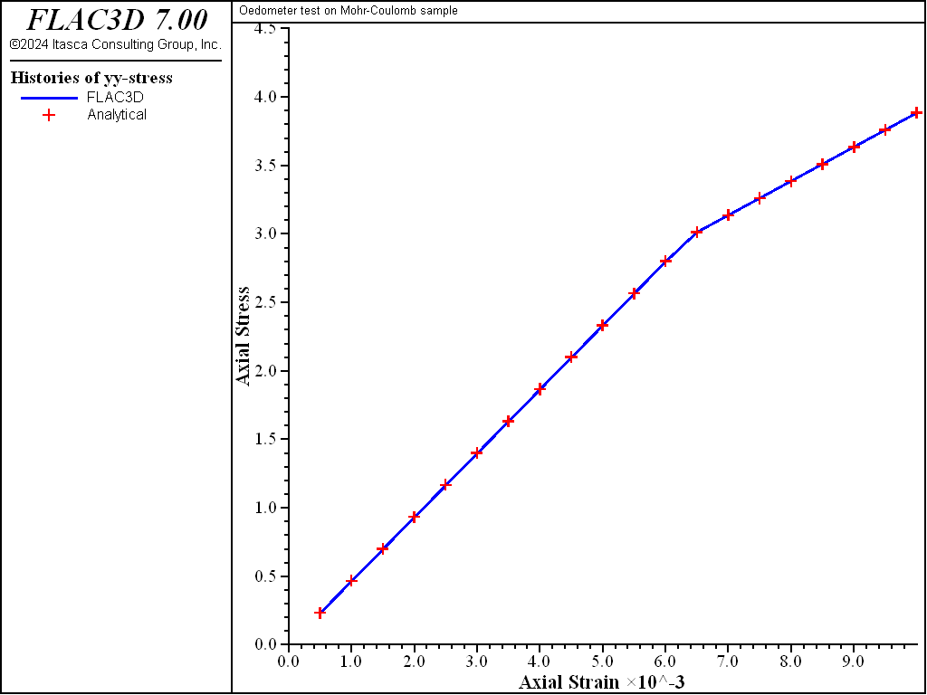
Figure 2: Oedometric test—comparison of numerical and analytical predictions for 10° dilation.
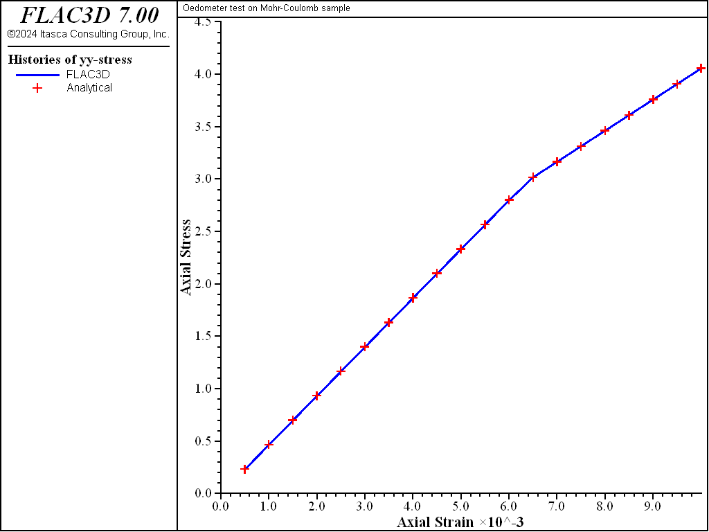
Figure 3: Oedometric test—comparison of numerical and analytical predictions for 0° dilation.
Data File
OedometerMohrCoulomb.dat
;---------------------------------------------------------------------
; oedometer test
; check plastic flow along an edge of the Mohr-Coulomb criterion
;---------------------------------------------------------------------
model new
model large-strain off
fish automatic-create off
zone create brick size 1 1 1
model title "Oedometer test on Mohr-Coulomb sample"
zone cmodel assign mohr-coulomb
zone property bulk 200 shear 200 co 1 friction 10 tension 5.67
[global vyv = -1.e-5]
program call 'oedometerTheoretical'
zone gridpoint fix velocity
zone gridpoint initialize velocity-y [vyv] range position-y 1.0
history interval 50
zone history displacement-y position 0 1 0
fish history n_sy
fish history a_sy
model save 'ini'
; --- dilation 10
zone property dil 10
[d_sigy]
model step 1000
model save 'dil10'
; --- dilation 0
model restore 'ini'
zone property dil 0
[d_sigy]
model step 1000
model save 'dil0'
Endnotes
| [1] | To view this project in FLAC3D, use the program menu.
⮡ FLAC |
| Was this helpful? ... | FLAC3D © 2019, Itasca | Updated: Feb 25, 2024 |