Overview
FLAC3D is a three-dimensional explicit Lagrangian finite-volume program for engineering mechanics computation. The basis for this program is the well-established numerical formulation used by our two-dimensional program, FLAC.[1] FLAC3D extends the analysis capability of FLAC into three dimensions, simulating the behavior of three-dimensional structures built of soil, rock, or other materials that exhibit path-dependent behavior.
Materials are represented by polyhedral elements within a three-dimensional grid that is adjusted by the user to fit the shape of the object to be modeled. Each element behaves according to a prescribed linear or nonlinear stress/strain law in response to applied forces or boundary restraints. The material can yield and flow, and the grid can deform (in large-strain mode) and move with the material that is represented.
The explicit, Lagrangian calculation scheme and the mixed-discretization zoning technique used in FLAC3D ensure that plastic collapse and flow are modeled very accurately. Because no matrices are formed, large three-dimensional calculations can be made without excessive memory requirements. The drawbacks of the explicit formulation (i.e., small timestep limitation and the question of required damping) are overcome by automatic inertia scaling and automatic damping that minimizes effects on the path to failure. FLAC3D offers an ideal analysis tool for the solution of three-dimensional problems in geotechnical engineering.
FLAC3D is designed specifically to operate on Microsoft Windows systems and is currently supported on Windows 7, Windows 8, and Windows 10. Calculations on realistically sized three-dimensional models in geo-engineering can be made in a reasonable time period. For example, a model containing 125,000 zones of a Mohr-Coulomb material can be generated within 600 MB RAM. The runtime to perform 5000 calculation steps for a 10,000 zone model of Mohr-Coulomb material is roughly 30 seconds on a 3.2 GHz Intel 6-Core i7 CPU.[#]_ The number of calculation steps required to reach a solution state with the explicit-calculation scheme can vary, but a solution typically can be reached within 3000 to 5000 steps for models containing up to 10,000 elements, regardless of material type. (The explicit-solution scheme is explained in the Theoretical Background section.) With the advancements in floating-point operation speed and the ability to install additional RAM at low cost, it should be possible to solve increasingly larger three-dimensional problems with FLAC3D.
The FLAC3D user interface includes both command-line (CLI) and graphical (GUI) capabilities. All aspects of program operation are available via the CLI in the i Console pane. Many but not all program operations can be performed in the program’s GUI components. Some operations (plotting, working with extrusions or building blocks, etc.) will be comparatively easier in the GUI components, and others may be invoked more efficiently (or necessarily) at the command line. Many FLAC3D commands will be similar or identical to those found in the Itasca program PFC, and both programs share a common command syntax and structure.
FLAC3D features accelerated 3D graphics that allow for rapid model visualization. Extensive plotting capabilities—including easy mechanisms for constructing animations (movies)—are available to facilitate pre- and post-processing.
A comparison of FLAC3D to other numerical methods, a description of general features and updates in FLAC3D Version 6.0, and a discussion of the program’s fields of application are provided in the topics that follow. If you wish to try FLAC3D right away, the best place to start is with the Tutorials.
The Lagrangian Finite Volume Grid
The Lagrangian finite volume grid spans the physical domain being analyzed. The smallest possible grid that can be analyzed with FLAC3D consists of only one zone. Most problems, however, are defined by grids that consist of hundreds, thousands, or millions of zones.
One FLAC3D zone is a hexahedron with eight vertices and six quadrilateral faces. Four other zone types are available (wedge, pyramid, d-brick, and tetrahedron), as degeneracies of this basic zone using fewer vertices and faces. See Zone for a discussion of zone data and conventions, and Theoretical Background for the theory, formulation, and implementation details.
The FLAC3D grid is specified in terms of global \(x\)-, \(y\)-, and \(z\)-coordinates. All gridpoints and zone centroids are located by their (\(x,y,z\)) position vector. A simple cubic grid is shown in the figure below. A set of ready-made (templatized) grids can be accessed from the menu option.
Every gridpoint and zone is identified by an identification number (ID), which can be used as a handle to refer to that specific object.
Grid generation with FLAC3D involves adjusting and shaping the mesh to fit the shape of the physical domain. The generation process may be performed in a variety of ways, such as using commands that build zones from primitive shapes, using the program’s interactive extrusion or building blocks facilities, or using advanced mesh generation techniques with third-party tools.
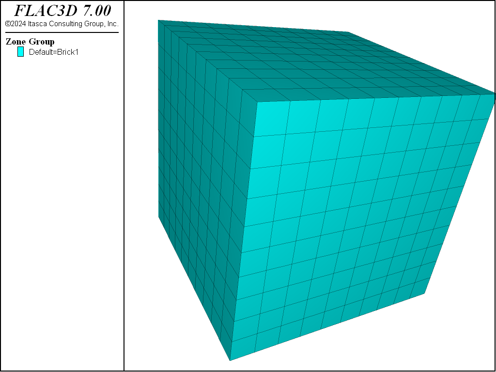
Figure 1: Finite volume grid with 1000 zones.
Nomenclature
FLAC3D uses nomenclature that is consistent, in general, with that used in conventional finite volume or finite element programs for stress analysis. The basic definitions of terms are reviewed here for clarification. The figure below illustrates the FLAC3D terminology.
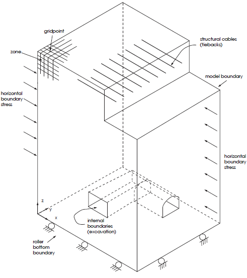
Figure 2: Example of a FLAC3D model.
- model
- The model (or FLAC3D model) is created by the user to simulate a physical problem. When referring to a FLAC3D model, the user implies a sequence of FLAC3D commands (see the FLAC3D Commands and FISH section) that define the problem conditions for numerical solution.
- zone
- The finite volume zone is the smallest geometric domain within which the change in a phenomenon (e.g., stress versus strain) is evaluated. Polyhedral zones of different shapes (e.g., brick, wedge, pyramid and tetrahedral-shaped zones) are used to create models and can be viewed upon plotting. Each polyhedral zone contains two overlaid sets of five tetrahedral subzones, but the user is not normally aware of these. Another term for zone is element, but this is generally reserved for structural elements for clarity.
- gridpoint
- Gridpoints are associated with the corners of the finite volume zones. There are four, five, six, seven, or eight gridpoints associated with each polyhedral zone, depending on the zone shape. A set of \(x\)-, \(y\)-, \(z\)-coordinates is assigned to each gridpoint, thus specifying the exact location of the finite volume zones. Other terms for gridpoint are nodal point and node, but these are generally reserved for structural elements for clarity.
- finite volume grid
- The finite volume grid is an assemblage of one or more finite volume zones across the physical region that is being analyzed. Another term for grid is mesh. The finite difference grid also identifies the storage locations of all state variables in the model. The procedure followed in FLAC3D is that, in general, all the vector quantities (e.g., forces, velocities, and displacements) are stored at gridpoint locations, while all scalar and tensor quantities (e.g., stress and material properties) are stored at zone centroid locations. See The Lagrangian Finite Volume Grid topic for more information.
- model boundary
- The model boundary is the periphery of the finite volume grid. Internal boundaries (i.e., holes within the grid) are also model boundaries.
- boundary condition
- A boundary condition is the prescription of a constraint or controlled condition along a model boundary (e.g., a fixed displacement or force for mechanical problems, an impermeable boundary for groundwater flow problems, adiabatic boundary for heat transfer problems, etc.).
- initial conditions
- This is the state of all variables in the model (e.g., stresses or pore pressures) prior to any loading change or disturbance (e.g., excavation).
- constitutive model
- The constitutive (or material) model represents the deformation and strength behavior prescribed to the zones in a FLAC3D model. Several constitutive models to assimilate different types of behavior commonly associated with geologic materials are available in FLAC3D. Constitutive models and material properties can be assigned individually to every zone in a FLAC3D model.
- null zone
- Null zones are zones that represent voids (i.e., no material present) within the finite volume grid.
- subgrid
- The finite volume grid can be composed of sub-grids. Sub-grids can be used to create regions of different shapes in the model (e.g., a dam sub-grid can be placed on a foundation sub-grid).
- attached faces
- Attached faces are grid faces of separated sub-grids that are attached or joined together. Attached faces must be coplanar and touching, but gridpoints on each face do not have to match. Sub-grids of different zone densities can be attached.
- interface
- An interface is a connection between sub-grids that can separate (e.g., slide or open) during the calculation process. An interface can represent a physical discontinuity such as a fault, contact plane, or interface between two different materials.
- range
- A range in a FLAC3D model is a filter that restricts the operations of a command to objects that fall within the definition of the filter. A range may or may not be associated with specific model objects (for example, a range specified in terms of ID numbers or groups will be associated with specific model objects, but a range specified in terms of \(x\)-, \(y\)-, and \(z\)-coordinates remains fixed in space, so the objects within it at one point of model processing may not be the same as the objects in it at a later point).
- range element
- A criterion in a range. Any range will have at least one range element, but may be composed of many range elements, may be designed to be a union or an intersection of the range elements supplied, and may invert any element provided by appending not at the end of the range element’s specification.
- group
- A group in a FLAC3D model refers to a name that can be assigned to one or more objects. Group names are assigned in a category, called slots, with the constraint that in a given object, each slot can only have one group assigned at a time. An object may have many different group names, each in different slots. As compared with a range, groups will always refer to specific model objects. Groups provide a way to persistently “name” parts of the model, and subsequently operate with ease on those parts of the model by applying that name to the range keyword in commands (e.g., consider zone cmodel assign mohr-coulomb range group "Layer1", which, as can be guessed, assigns the Mohr-Coulomb model to the zones in the group “Layer1”).
- id number
Individual elements of a FLAC3D model are identified by identification (ID) numbers. Almost all model elements have ID numbers, including interfaces, gridpoints, zones, histories, tables, and structural element entities (i.e., beams, cables, piles, shells, liners, and geogrids). These are unique numbers that are assigned by the code allowing the user to identify specific elements in a model. Elements that have IDs supply a list keyword that is used to return ID-sorted data about the object (for example, try
zone list information).Component identification (component-id) numbers are also assigned to individual elements of a structural element entity. A unique component-id number is created for each node, element, and node/grid link that make up a beam, cable, pile, shell, liner, or geogrid entity.
- names
- For certain types of model element objects (like histories, tables, or interfaces) it is convenient to assign a clear short user-assigned name to an object so it can be referred to later. In general, this is done using a name, which is normally assigned when the object is created. A name is meant to be a short identifying string, although technically it can be of any length. As a special case, an integer can be used on the command line as a name, in which case it will be converted automatically into a string.
- structural element
Two types of structural elements are available in FLAC3D. Two-noded, linear elements represent the behavior of beams, cables, and piles. Three-noded, flat triangular elements represent shells, liners, and geogrids. Structural elements are used to simulate the interaction of structural support within a soil or rock mass. Nonlinear material behavior can be represented with some of the elements.
Each structural element entity (beam, cable, pile, shell, liner, or geogrid) is composed of three components: nodes; individual elements; and node/grid links. The characteristics of each of these components distinguish the behavior of the beam, cable, pile, shell, liner, and geogrid entities.
- step
- Because FLAC3D is an explicit code, the solution to a problem requires a number of computational steps. During computational stepping, the information associated with the phenomenon under investigation is propagated across the zones in the finite volume grid. A certain number of steps is required to arrive at an equilibrium (or steady-flow) state for a static solution. Typical problems are solved within 2000 to 4000 steps, although large complex problems can require tens of thousands of steps to reach a steady state. When using the dynamic analysis option,
model steprefers to the actual timestep for the dynamic problem. Other terms for step are timestep and cycle. - static solution
- A static or steady-state solution is reached in FLAC3D when the rate of change of kinetic energy in a model approaches a negligible value. This is accomplished by damping the equations of motion. At the conclusion of the static solution stage, the model will either be at a state of equilibrium or at a state of steady flow of material if a portion (or all) of the model is unstable (i.e., fails) under the applied loading conditions. This is the default calculation in FLAC3D.[2] Static mechanical solutions can be coupled to transient groundwater flow or heat transfer solutions. (As an option, fully dynamic analysis can also be performed by inhibiting the static solution damping.)
- unbalanced force
- The unbalanced force indicates when a mechanical equilibrium state (or the onset of plastic flow) is reached for a static analysis. A model is in exact equilibrium if the net nodal-force vector (the resultant force) at each gridpoint is zero. The maximum nodal-force vector is monitored in FLAC3D and printed to the screen when the
model stepormodel solvecommand is invoked. The maximum nodal force vector is also called the unbalanced or out-of-balance force. The maximum unbalanced force will never exactly reach zero for a numerical analysis, but the model is considered to be in equilibrium when the maximum unbalanced force is small compared to the total applied forces in the problem. If the unbalanced force approaches a constant nonzero value, this probably indicates that failure and plastic flow are occurring within the model. When a gridpoint is fixed in a given direction, the component of the unbalanced force in that direction is equivalent to the reaction force. - dynamic solution
- For a dynamic solution, the full dynamic equations of motion (including inertial terms) are solved; the generation and dissipation of kinetic energy directly affect the solution. Dynamic solutions are required for problems involving high frequency and short duration loads (e.g., seismic or explosive loading). The dynamic calculation is an optional module for FLAC3D (see Dynamic Analysis).
- large strain/small strain
- By default, FLAC3D operates in small-strain mode; gridpoint coordinates are not changed even if computed displacements are large (compared to typical zone sizes). In large-strain mode, gridpoint coordinates are updated at each step according to computed displacements. In large-strain mode, geometric nonlinearity is possible.
- project
- A project refers to the collection of data files and other inputs, and save files and other outputs, that comprise a FLAC3D model. A project so-defined is stored in a project file. The terms “project” and “project file” are so nearly synonymous that they are likely to be used somewhat interchangeably in this documentation.
- primitive
- A templatized shape that can be used with the
zone createcommand to create a range of FLAC3D grids. The shapes are keywords of the command; refer to the reference information on the command for details on primitives. - element
- See zone.
- mesh
- See finite volume grid.
- console
- A generic reference to the Console pane in FLAC3D.
- Console pane
- This pane is divided into two parts. The lower part of the pane is the command prompt, where users may enter commands one at a time. The upper part of the pane (variously referred to as the output, the output window, the console output, etc.) echoes commands and prints written output resulting from command processing. The Options dialog provides options for which output and how much of it will be displayed in the output.
- command prompt
- The lower portion of the Console pane, which can be used to enter commands line by line.
Endnotes
| [1] | Itasca Consulting Group Inc. FLAC (Fast Lagrangian Analysis of Continua), Version 8.0, 2014. .. [#] See [need a link here to runtime comparison] |
| [2] | In some finite element (FE) literature, there is the mistaken notion that a dynamic solution method cannot produce a true equilibrium state, compared to an FE solution, which is believed to perfectly satisfy the set of governing equations at equilibrium. In fact, both methods only satisfy the equations approximately, but the level of residual errors can be made as small as desired. In FLAC3D, the level of error is objectively quantified as the ratio of unbalanced force at a gridpoint to the mean of the set of absolute forces acting at the gridpoint. This measure of error is very similar to the convergence criteria used in FE solutions. In both cases, the solution process is terminated when the error is below a desired value. |
| Was this helpful? ... | FLAC3D © 2019, Itasca | Updated: Feb 25, 2024 |