Grid Generation
FLAC3D has three main built-in methods for creating zones for grids: primitives, extrusions, and building blocks. Each is different. Each offers distinct advantages and disadvantages. For initial generation of grids, they are mutually exclusive (i.e., you cannot create one set of zones using primitives and an extrusion at the same time). However, the program offers commands that allow zones from any method to be further modified, combined, and so forth, as needed. The right path to the geometry of a model might involve an adept combination of these methods of zone generation.
In addition, FLAC3D can create zones from imported files. Third-party tools (volume-based CAD programs such as Rhino) can be combined with Itasca’s advanced automatic mesher Griddle to create zones as well. This last is the most advanced approach to zone creation, suitable for the most complex meshes for which FLAC3D’s build-in tools are either insufficient or excessively labor intensive.
FLAC3D also has additional facilities for generating and modifying zones. For circumstances where geometry is complex but exact conformance of zone faces to surfaces is not physically significant, it is common to create octree meshes using geometric descriptions and mesh densification, as shown briefly in Geometry-Based Densification: Octree Meshing. Where there are complex unintersecting layers, or uneven surface topography, the zone generate from-topography command can be used as illustrated in Surface Topography and Layering.
This section describes the use of the built-in methods of grid generation and briefly describes the additional capabilities provided by third-party tools and imports. The considerations involved with grid generation are extensive. Selection of the right mesh generation method and the efficient deployment of that method is a critical part of the FLAC3D modeling process.
As can be intuited from the number of tools FLAC3D makes available, there is no single mesh generation method that is the best answer for every case. The optimal approach is very dependent on the model geometry and the goals of the analysis. The following is a brief initial guide for which built-in methods should be chosen:
- If the problem has very simple, regular geometry, or one that happens to conform to one of the shapes available to the
zone createcommand, then the primitive approach is the fastest and easiest. - If the geometry of the problem can be described in a two-dimensional diagram, or with only minor variations in the third dimension, then the extrusion should be considered first. Note that 2D starting geometry can be exported to Building Blocks for 3D modifications.
- If the problem is more complex but still consists of relatively regular shapes, then Building Blocks should be considered. This is fairly common for civil engineering problems involving tunnels, structures, or foundations. Irregular shapes can be accommodated with this tool with either extensive manual adjustment or by strategic use of the draping tool, but this is recommended only for limited areas in an otherwise regular model.
- If the problem is very irregular and/or involves complex irregular intersecting surfaces, then one needs to decide if exact conformation of the zone faces to the surfaces describing the model is important to the result. Often, for irregular orebodies or other material boundaries, this is not important to the overall physical response of the model. In this case, using an octree approach (perhaps after first using Building Blocks to create the area of most interest) is often used. This type of model is not uncommon in mining.
- If the problem is very irregular and exact conformance of the mesh is important, then Itasca’s Griddle or another third-party meshing tool should be considered.
By any means of construction, grid generation involves tradeoffs between computational efficiency, realism of model geometry, and accuracy of results. The following factors govern those tradeoffs.
Hexahedral zones are preferable because:
- the mixed-discretization procedure makes them respond more accurately to situations involving constant-volume plastic deformation (e.g., as seen during Mohr-Coulomb shear failure); and
- the mixed-discretization procedure makes their response more accurate in general (slightly higher-order response).
However, they are more difficult to use than tetrahedral zones when building geometrically complex models.
Computational speed decreases with the number of zones.
Finer meshes lead to more accurate results in that they provide a better representation of high-stress gradients.
Accuracy increases as zone aspect ratios tend to unity.
If different zone sizes are needed, then the more gradual the change from the smallest to the largest, the better the results.
Primitive-Based Grids
At first pass, it may seem that the primitive-based grid generation of FLAC3D is limited to rather simple, regular-shaped regions. In the introductory sections, the examples provided are often uniform, polyhedral grids. FLAC3D primitive shapes, however, can be distorted to fit arbitrary and complicated volumetric regions. FLAC3D provides powerful grid generation commands to manipulate primitives to fit various shapes of three-dimensional problem domains.
The procedure for implementing primitive-based grids by command is described in this topic. An overview of the operation is given first, in Overview of the Grid Generator. This is followed, in Fitting the Grid to Simple Shapes and Grid Generation with FISH, by presentations on various aspects of grid generation, along with guidelines to follow in designing the grid for accurate solutions. Examples are given to illustrate each aspect.
One important aspect in grid generation is that all physical boundaries to be represented in the model simulation (including regions that will be added, or excavations created at a later stage in the simulation) must be defined before the solution stepping begins. Shapes of structures that will be added later in a sequential analysis must be defined and then removed (via either zone cmodel assign null or zone delete) until they are to be activated. The purpose of the grid generator is to facilitate the creation of all required physical shapes in the model.
All examples listed in the section are included in the project file “grid-generation.prj”.
Overview of the Grid Primitives
Grid generation using primitives in FLAC3D involves patching together grid shapes of specific connectivity to form a complete model with the desired geometry. Several types of primitives are available, and these can be connected and conformed to create complex three-dimensional geometries.
The generation of zones for each primitive type is performed with the zone create command. Single reference points can be defined using the zone gridpoint create command to put gridpoints at specific locations and subsequently refer to them in the zone create command. The zone gridpoint merge command can be used to ensure that separate primitives are connected properly. All gridpoints along matching faces of zone primitives must fall within a specified tolerance for two primitives to be merged. Alternatively, the zone attach command is available to connect primitive meshes of different zone sizes. FISH can be used to adjust the final mesh, if necessary, to conform to the surfaces of the model region. The following sections describe the use of each of these facilities to create a FLAC3D mesh.
Zone Generation
The primitive-based FLAC3D grid is generated with the zone create command. This command actually accesses a library of primitive shapes; each shape has a specific type of grid connectivity. The primitive shapes available in FLAC3D, listed in order of increasing complexity, are as follows.
| Keyword | Definition |
|---|---|
| brick | brick-shaped mesh |
| wedge | wedge-shaped mesh |
| uniform-wedge | uniform wedge-shaped mesh |
| tetrahedron | tetrahedral-shaped mesh |
| pyramid | pyramid-shaped mesh |
| cylinder | cylindrical-shaped mesh |
| degenerate-brick | degenerate brick-shaped mesh |
| radial-brick | radially graded mesh around brick |
| radial-tunnel | radially graded mesh around parallelepiped-shaped tunnel |
| radial-cylinder | radially graded mesh around cylindrical-shaped tunnel |
| cylindrical-shell | cylindrical shell mesh |
| cylindrical-intersection | intersecting cylindrical-shaped tunnels |
| tunnel-intersection | intersecting parallelepiped-shaped tunnels |
As was seen in Tutorial: Illustrative Model — Mechanics of Using FLAC3D, zone create commands can be used alone to create a zoned model. If the 3D domain consists of simple shapes, the primitives can be applied individually or connected together to create the FLAC3D grid.
As an example, a quarter-symmetry model can be created for a cylindrical tunnel with the command
zone create radial-cylinder size 5 10 6 12 fill
The size keyword defines the number of zones in the grid. For the cylindrical tunnel, each entry following the size keyword corresponds to the number of zones in a specific direction. In this case, there are five zones along the inner radius of the cylindrical tunnel, ten zones along the axis of the tunnel, six zones along the circumference of the tunnel, and twelve zones between the periphery of the tunnel and the outer boundary of the model. The image below shows the model grid. The fill keyword is given to fill the tunnel with zones.
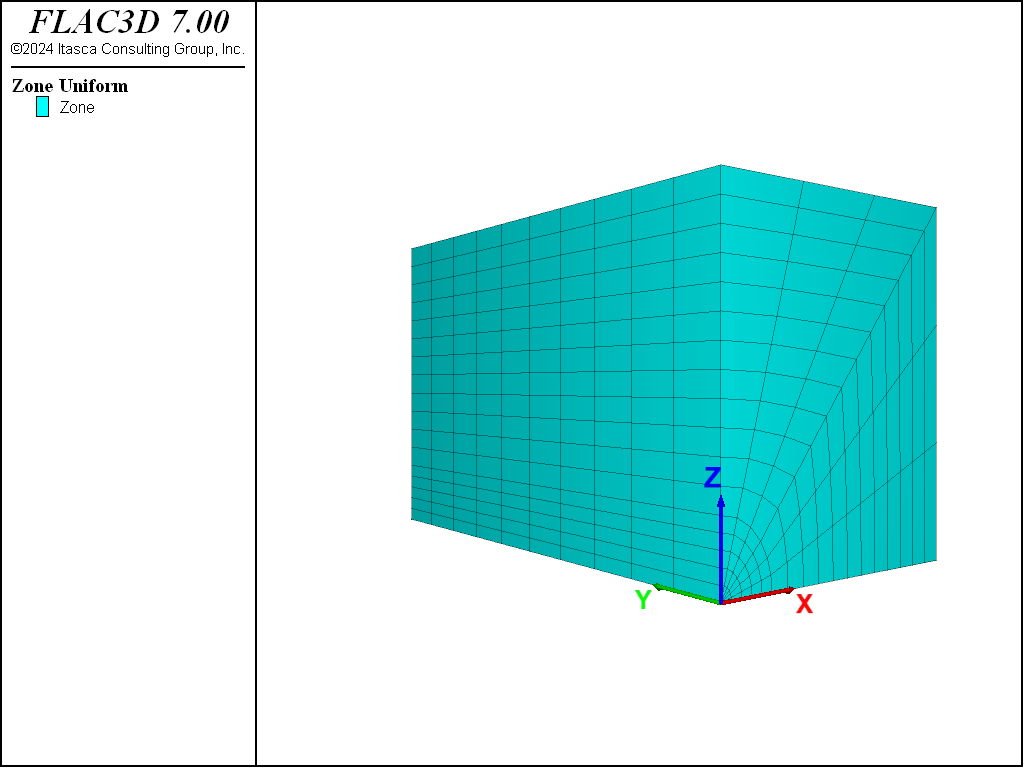
Figure 1: Grid of cylindrical tunnel model.
In addition to size and fill, there are several other keywords available to define the characteristics of the primitive shapes. The available characteristic keywords for primitive shapes are summarized in the table below. Refer to the zone create command and the reference diagrams it contains to identify which keywords and numerical entries are applicable for each primitive shape. For example, click the thumbnail on zone create radial-cylinder to see the order in which the size entries (i1, i2, i3, i4) should be entered for the cylindrical tunnel.
| Keyword | Definition |
|---|---|
| dimension | dimensions (length) of interior regions |
| edge | edge length for the sides of the mesh |
| fill | fill the interior region with zones |
| point | reference (corner) points for the shape. First should follow a point index ( 0 through 16 ) and then an \(x,y,z\) coordinate location. |
| ratio | geometric ratio used to space zones |
| size | number of zones for each shape |
The ratio keyword is of particular significance when designing a grid to provide an accurate solution without requiring an excessive number of zones. For example, if fine zoning is required immediately around the periphery of the cylindrical tunnel in order to provide a more accurate representation of high-stress gradients, ratio can be used to adjust the zone size to be small close to the tunnel, and gradually increase in size away from the tunnel.
To see the effects of using the ratio keyword, type the command
zone create radial-cylinder size 5 10 6 12 ratio 1 1 1 1.2
Each size entry is controlled by a ratio. In this example, the fourth size entry has a geometric ratio of 1.2 (i.e., each successive zone is 1.2 times larger than the preceding zone, moving from the tunnel periphery to the outer boundary—see the next figure). A ratio smaller than 1.0 can be given to change from an increasing to a decreasing geometric ratio.
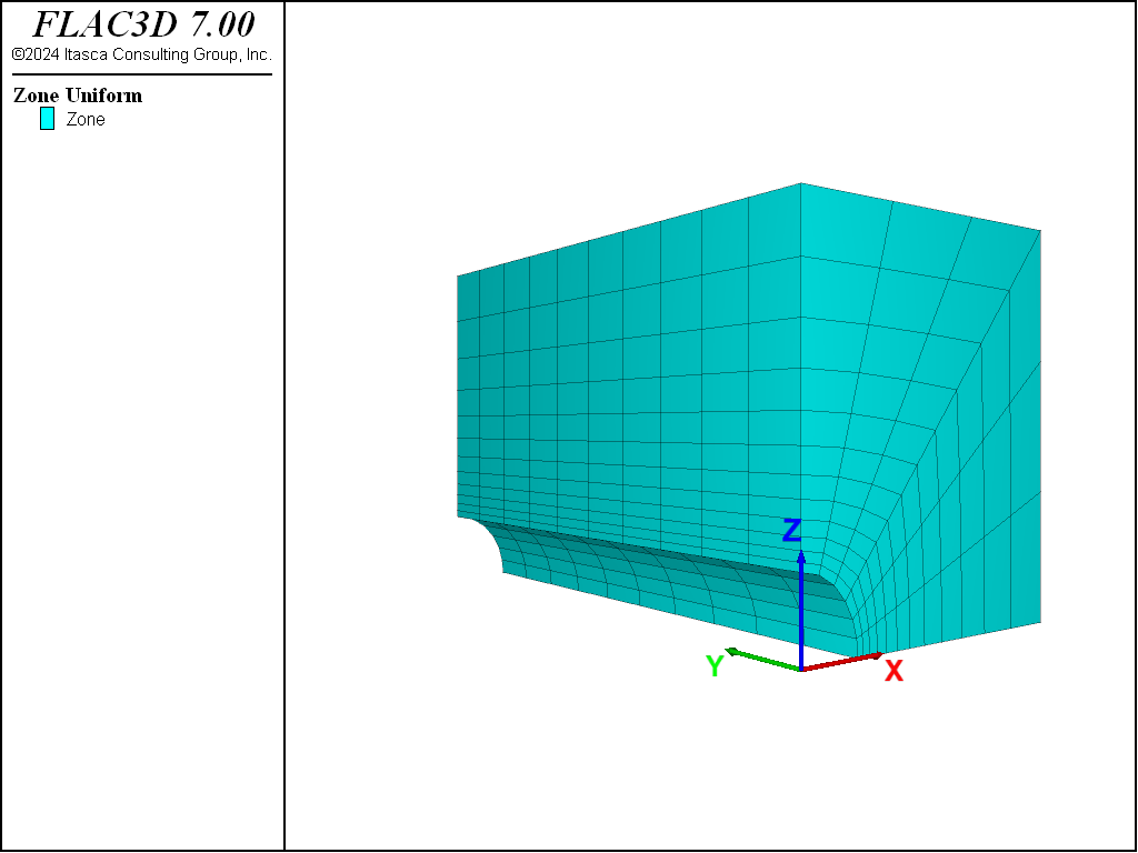
Figure 2: Radially graded grid around cylindrical tunnel.
Sizing the grid for accurate results, but with a reasonable number of zones, can be complicated. Three factors should be remembered:
- Finer meshes lead to more accurate results in that they provide a better representation of high-stress gradients.
- Accuracy increases as zone aspect ratios tend to unity. A rule of thumb is try to avoid aspect ratios greather than 10 or so.
- If different zone sizes are needed, then the more gradual the change from the smallest to the largest, the better the results.
The examples in the following sections illustrate some applications of these factors.
Several zone create commands can be given to connect two or more primitive shapes together to build a grid. For example, to build a horseshoe-shaped tunnel, the radial-cylinder and radial-tunnel shapes can be used as demonstrated in this example:
Building a horseshoe-shaped tunnel — half model
zone create radial-cylinder size 5 10 6 12 rat 1 1 1 1.2 ...
     point 0 (0,0,0) point 1 (100,0,0) point 2 (0,200,0) point 3 (0,0,100)
zone create radial-tunnel size 5 10 5 12 rat 1 1 1 1.2 ...
     point 0 (0,0,0) point 1 (0,0,-100) point 2 (0,200,0) point 3 (100,0,0)
Refer to the reference figures for zone create radial-cylinder and zone create radial-tunnel when building these shapes. The model boundary dimensions are 100 × 200 × 100; the boundary coordinates are defined with point keywords. The grid is shown below. Note that the radial-tunnel shape is turned 90° to fit beneath the radial-cylinder shape. This is accomplished by specifying different point coordinate entries for the radial-tunnel shape.
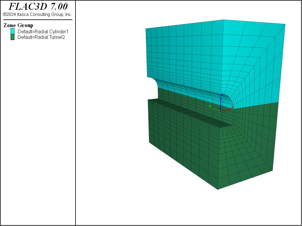
Figure 3: Horseshoe-shaped tunnel made from radcylinder and radtunnel primitives.
With zone create, two additional options are available to assist with the creation of a grid composed of multiple shapes: zone copy and zone reflect. The former is used to copy a shape or shapes to a new position by adding an offset vector to all the gridpoints. The latter is used to reflect the shape or shapes across a symmetry plane. The next example shows the additional command needed to reflect the geometry created by the earlier commands.
Building a horseshoe-shaped tunnel — full model
zone create radial-cylinder size 5 10 6 12 rat 1 1 1 1.2 ...
     point 0 (0,0,0) point 1 (100,0,0) point 2 (0,200,0) point 3 (0,0,100)
zone create radial-tunnel size 5 10 5 12 rat 1 1 1 1.2 ...
     point 0 (0,0,0) point 1 (0,0,-100) point 2 (0,200,0) point 3 (100,0,0)
zone reflect dip 90 dip-direction 270 origin (0,0,0)
The resulting grid is shown below. The symmetry plane is a vertical plane (located by the dip, dip-direction, and origin keywords) coincident with the \(x\) = 0 plane. Note that dip angle (dip) and dip direction (dip-direction) assume that \(x\) corresponds to “East,” \(y\) to “North”, and \(z\) to “Up.”
A third option, the zone gridpoint create command, is available to position single points in the model region. This is useful for positioning reference points of primitives. The section Fitting the Grid to Simple Shapes below presents an example use of zone gridpoint create to position the invert of two tunnels of different sizes at the same elevation.
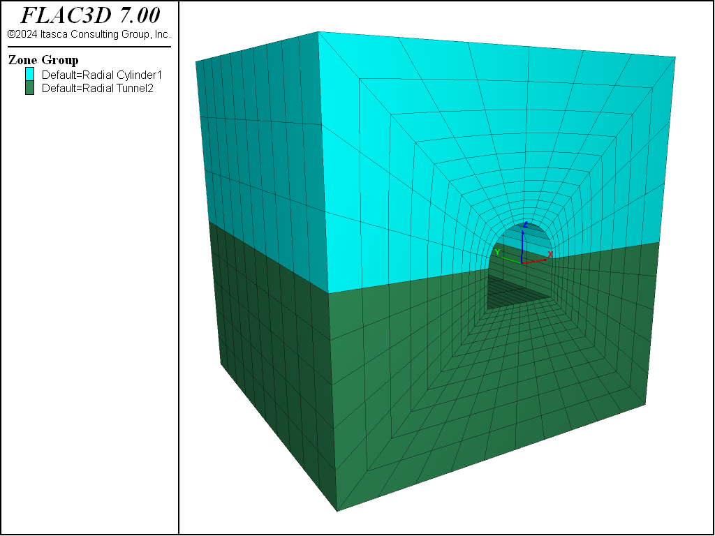
Figure 4: Complete horseshoe-shaped tunnel made from the reflect keyword.
Connecting Adjoining Primitive Shapes
When building a geometry out of primitives, the sides of the primitives must connect to form an unbroken continuum. During execution of a zone create command, a check is made for each boundary gridpoint against the boundary gridpoints of zones that already exist. Internal gridpoints are not checked. If two boundary gridpoints fall within a tolerance of 1 × 10⁻⁷ (relative to the magnitude of the gridpoints position vector) of each other, they are assumed to be the same point, and the first gridpoint is used instead of creating a new one for all subsequent calculations.
The user is responsible for ensuring that all gridpoints along adjoining primitives correspond to one another. The use of reference points with the command zone gridpoint create during model creation can be useful to make sure that the bounding brick is specified correctly for both primitives. Make sure that the number of zones is correct and that the ratios used for the zone distribution are consistent. Note that if the ratio for one primitive is going the opposite direction of the other, the inverse ratio should be used for one of the primitives to ensure that boundary gridpoints match.
This version of FLAC3D does not issue a warning message if gridpoints at boundaries do not match. Localized velocity anomalies will be observed at nonmatching gridpoints in the model when the calculation is started. If it is discovered that some gridpoints don’t match, the zone gridpoint merge command can be used to merge these gridpoints after the zone create command has been applied.
The zone attach command can be used to connect primitives with different zone sizes. There are some restrictions, though, to the range in zone size that may be specified with this approach. For the most accurate calculations, the ratio of zone sizes should be a multiple integer ratio (e.g., 2 to 1, 3 to 1, 4 to 1). It is recommended that the ratio be tested first by running the model under elastic conditions. If a discontinuity is observed in the displacement, or stress distribution across the attached grids, then the ratio of zone sizes may need to be adjusted. However, if the discontinuity is small and far from the region of interest, it may not have a significant influence on the calculation.
The next example illustrates the use of the zone attach command and the effect of different zone sizes. A brick primitive with a zone dimension of 0.5 is connected to a brick primitive with a zone dimension of 1. The resulting \(z\)-displacement contours are shown in the next figure below.
In the next example, alternatively, the first two command lines can be changed to
zone create brick size 4 4 4
zone densify segments 2 range position-x 2 4
where zone densify segments 2 refines the upper zones (between the \(z\)-coordinate of 2 and 4) with the segment number of 2 on each edge.
Two unequal sub-grids
model large-strain off
zone create brick size 4 4 2 point 0 (0,0,0) point 1 (4,0,0) ...
                             point 2 (0,4,0) point 3 (0,0,2)
zone create brick size 8 8 4 point 0 (0,0,2) point 1 (4,0,2) ...
                             point 2 (0,4,2) point 3 (0,0,4)
zone attach by-face range position-z 2
zone cmodel assign elastic
zone property bulk 8e9 shear 5e9
zone gridpoint fix velocity-z range position-z 0
zone gridpoint fix velocity-x range union position-x 0 position-x 4
zone gridpoint fix velocity-y range union position-y 0 position-y 4
zone face apply stress-zz -1e6 range position-z 4 position-x 0,2 position-y 0,2
model history mechanical unbalanced-maximum
model solve
model save 'att'
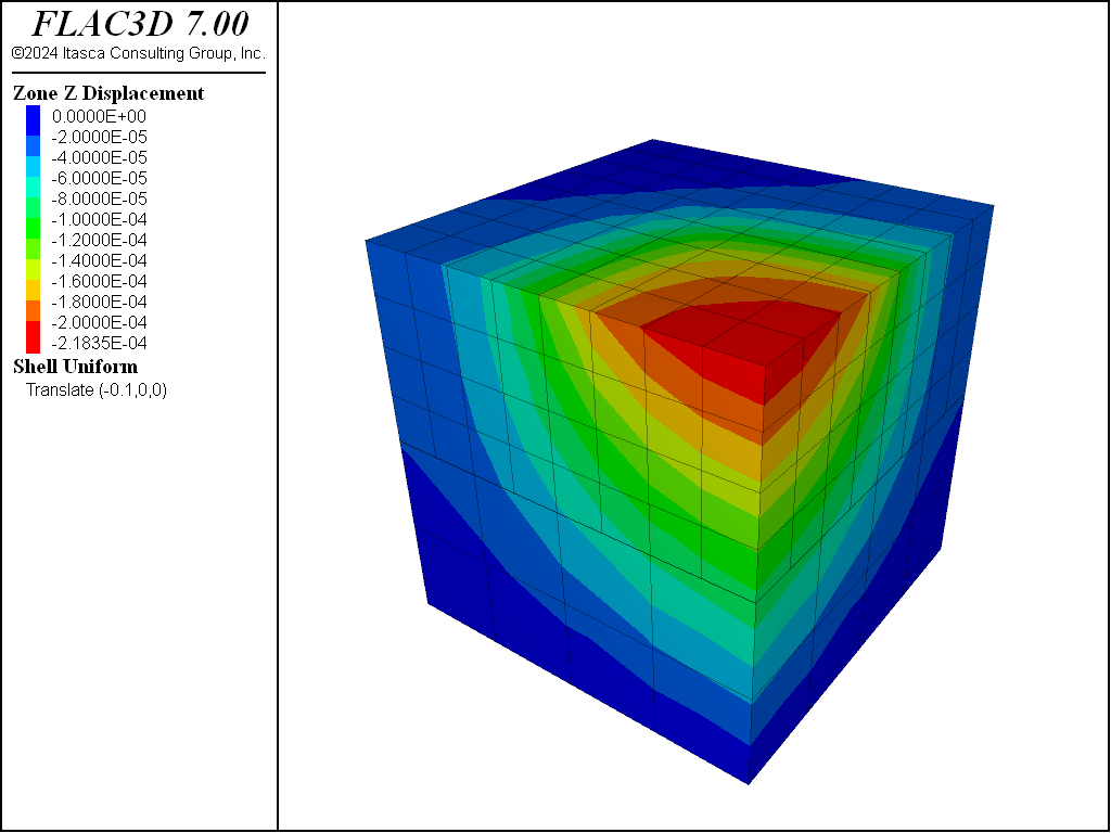
Figure 5: z-displacement contours in two attached grids with zone ratio of 2 to 1.
To test the accuracy, a similar run is performed, but for a single grid with a constant zone dimension of 0.5. The data file is given next. The results are shown in the figure that follows. This plot is almost identical to the one above.
A single grid for comparison to two sub-grids
model large-strain off
zone create brick size 8 8 8 point 0 0,0,0 point 1 4,0,0 ...
                             point 2 0,4,0 point 3 0,0,4
zone cmodel assign elastic
zone property bulk 8e9 shear 5e9
zone gridpoint fix velocity-z range position-z 0
zone gridpoint fix velocity-x range union position-x 0 position-x 4
zone gridpoint fix velocity-y range union position-y 0 position-y 4
zone face apply stress-zz -1e6 range position-z 4 position-x 0,2 position-y 0,2
model history mechanical unbalanced-maximum
model solve
model save 'noatt'
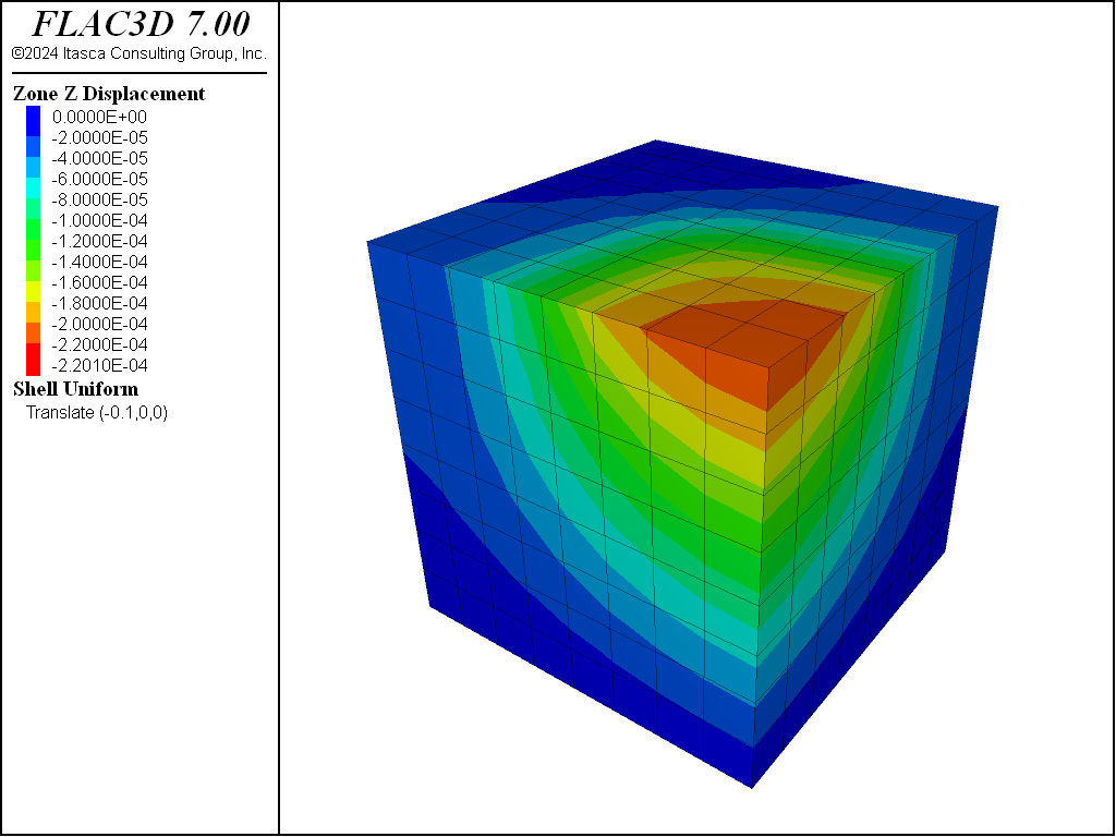
Figure 6: z-displacement contours in single grid.
Fitting the Grid to Simple Shapes
The intention of grid generation is to fit the model grid to the physical region under study. For simple geometries, the zone create command is all that is required to generate a model grid to fit the problem domain. To determine whether zone create is sufficient, try defining the problem domain by one or more of the primitive shapes shown in the command’s documentation.
For example, consider a problem geometry involving three parallel tunnels (a service tunnel located midway between two larger main tunnels). The three tunnels are all cylindrical in shape, so the radial-cylinder primitive shape is the logical choice to build the tunnel grids. A vertical symmetry plane may be assumed to exist along the centerline of the service tunnel. Thus, it is only necessary to create a mesh for one main tunnel and half of the service tunnel.
Note
This example is presented as an illustration of more advanced primitive zone creation techniques. In practice, it is recommended that geometry like this be created with the 2D Extruder.
There are two important concerns when building any model: 1) the density of zoning required for an accurate solution in the region of interest; and 2) how the location of the grid boundaries influence model results.
It is important to have a high density of zoning in regions of high stress- or strain-gradients. Often, it is possible to perform two-dimensional analyses to define these regions. For this problem, a 2D FLAC calculation can easily be run to determine an acceptable density of zones around the tunnels. For demonstration purposes, a zone size is selected that is roughly one-half the service tunnel radius for the zones surrounding the tunnels.
The first step in grid generation for this problem is to use radial-cylinder primitives to create the grids for the tunnels. The complicating factor is that the tunnels are of different sizes and have the same invert elevation. The service tunnel has a radius of 3 m, and the main tunnels have a radius of 4 m. The length of the model corresponds to a 50 m length of the tunnels. The following example shows the commands to create the grid surrounding the tunnels.
Creating a grid for two tunnels with the same invert elevation
; main tunnel
zone create radial-cylinder point 0 (15,0,0)  point 1 (23,0,0) ...
                            point 2 (15,50,0) point 3 (15,0,8) ...
                            size 4 10 6 4 dim 4 4 4 4 rat 1 1 1 1 fill ...
                            group 'service'
zone reflect dip 90 dip-direction 90 origin (15,0,0)
zone reflect dip 0 origin (0,0,0)
; service tunnel
zone gridpoint create (2.969848, 0.0,-0.575736) name 'p2124'
zone gridpoint create (2.969848,50.0,-0.575736) name 'p2125'
zone create radial-cylinder point 0 (0, 0,-1) point 1 (7,0,0) ...
                            point 2 (0,50,-1) point 3 (0,0,8) ...
                            point 4 (7,50,0)  point 5 (0,50, 8) ...
                            point 6 (7,0,8)   point 7 (7,50, 8) ...
                            point 8 gridpoint 'p2124' ...
                            point 10 gridpoint 'p2125' ...
                            size 3 10 6 4 dim 3 3 3 3 rat 1 1 1 1
zone create radial-cylinder point 0 (0, 0,-1) point 1 (0,0,-8) ...
                            point 2 (0,50,-1) point 3 (7,0,0) ...
                            point 4 (0,50,-8) point 5 (7,50, 0) ...
                            point 6 (7,0,-8) point 7 (7,50,-8) ...
                            point 9 gridpoint 'p2124' ...
                            point 11 gridpoint 'p2125' ...
                            size 3 10 6 4 dim 3 3 3 3 rat 1 1 1 1
The main tunnel grid is created first: one-quarter of the grid is generated; then the grid is reflected across horizontal and vertical planes to create the grid for the entire tunnel. The reflect option cannot be used for the service tunnel, because the invert of the service tunnel is required to be at the same elevation as the main tunnel. The vertices locating the service tunnel radius must be adjusted in the radial-cylinder primitive. This is done by first defining these locations using the
zone gridpoint create command. The corner points point 8 and point 10 in one radial-cylinder primitive, and point 9 and point 11 in the other primitive, are located at the reference points. This ensures that the two primitives will match at boundary gridpoints when the grid is generated. The figure below shows the grid for the tunnels. The vertical plane at \(x\) = 0 is a symmetry plane.

Figure 7: Inner grid for the service and main tunnels.
Note
*This creates a liner that is rigidly attached to the grid. A liner with a connection to the grid that can slide/separate can be specified with the structure liner create command.
This model begins with the main tunnel filled with zones and the service tunnel not filled. The excavation and construction stages analyzed with this model are described later in this topic. Before the main tunnel is excavated, a liner is defined for the service tunnel. This is accomplished with the structure shell create command, which creates a tunnel lining composed of structural shell elements.* Structural elements should generally be used to represent thin tunnel liners because they provide a more accurate representation of liner bending than a liner composed of finite-difference zones. See the section Structural Elements for detailed information on the structural element logic in FLAC3D. The next example gives the command to create the liner.
Creating a liner in the service tunnel
; liner
structure shell create by-zone-face range cylinder ...
                                     end-1 (0,0,-1) end-2 (0,50,-1) ...
                                     radius 3
The liner contains 240 structural shell elements and is connected to the FLAC3D grid at 143 structural-node links. The grid with the liner is shown below.
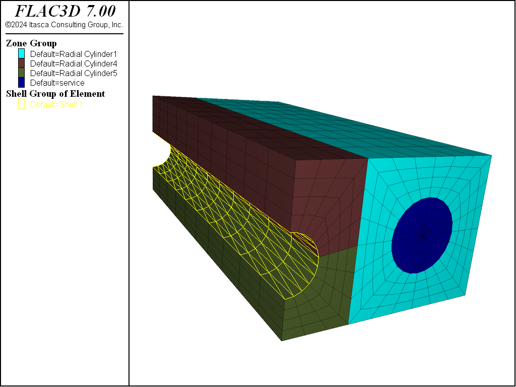
Figure 8: Liner elements in service tunnel.
Finally, the outer-boundary grid is created around the tunnel grid. For analyses of underground excavations, boundaries should be located roughly ten excavation diameters from the excavation periphery. The distance, however, can vary depending on the purpose of the analysis. If failure is of primary concern, then the model boundaries may be closer; if displacements are important, then the distance to the boundaries may need to be increased.
It is important to experiment with the model to assess boundary effects. Begin with a coarse two-dimensional grid, using FLAC, and bracket the boundary effect using fixed and free boundary conditions while changing the distance to the boundary. The resulting effect of changing the boundary can then be evaluated in terms of differences in stress or displacement calculated in the region of interest. The boundary location should then be tested with a coarse grid in FLAC3D.
The boundary grid is created with the radial-tunnel and brick primitives for this model. The zone reflect command is used to reflect the grid across the plane at \(z\) = 0. The range keyword is used to restrict the action of zone reflect. See the following example.
The final grid for this problem is shown below.
Creating the boundary grid
; outer boundary
zone create radial-tunnel point  0 ( 7, 0, 0) point  1 (50, 0, 0) ...
                          point  2 ( 7,50, 0) point  3 (15, 0,50) ...
                          point  4 (50,50, 0) point  5 (15,50,50) ...
                          point  6 (50, 0,50) point  7 (50,50,50) ...
                          point  8 (23, 0, 0) point  9 ( 7, 0, 8) ...
                          point 10 (23,50, 0) point 11 ( 7,50, 8) ...
                          size 6 10 3 10 ratio 1 1 1 1.1
zone create brick point 0 ( 0, 0, 8) point 1 ( 7, 0, 8) ...
                  point 2 ( 0,50, 8) point 3 ( 0, 0,50) ...
                  point 4 ( 7,50, 8) point 5 ( 0,50,50) ...
                  point 6 (15, 0,50) point 7 (15,50,50) ...
                  size 3 10 10 ratio 1 1 1.1
zone reflect dip 0 origin (0,0,0) ...
                   range position-x 0 23 position-y 0 50 position-z 8 50
zone reflect dip 0 origin (0,0,0) ...
                   range position-x 23 50 position-y 0 50 position-z 0 50
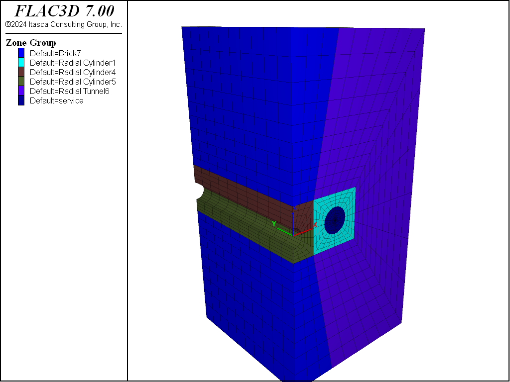
Figure 9: Complete grid for service and main tunnels.
Grid Generation with FISH
FISH can be used to specify a geometric shape that is not readily available by using the built-in primitives in FLAC3D. It is also possible to create your own primitive shapes using FISH. The following example constructs a radially graded mesh around a spherical cavity. Only one-eighth of the grid is generated. The grid can be reflected to create the complete spherical cavity.
A radial-brick primitive is the basis for creating our “radsphere” shape. First, parameters that describe the sphere within a cube are defined: the radius of the spherical cavity; the length of the outer cube edge; the number of zones along the outer cube edge; and the number of zones in the radial direction from the inner cube to the outer cube. Then a radial-brick is defined such that the spherical cavity will be inscribed in the inner cube. The next example lists the commands to create the initial grid for a geometric ratio of 1.2. The grid is shown in the figure that follows.
Parameters to create a radially graded mesh around a spherical cavity
[global rad=4.0    ] ; radius of spherical cavity
[global len=10.0   ] ; length of outer box edge
zone create radial-brick edge [len] size 6,6,6,10 ...
                         rat 1.0 1.0 1.0 1.2 dim [rad] [rad] [rad]
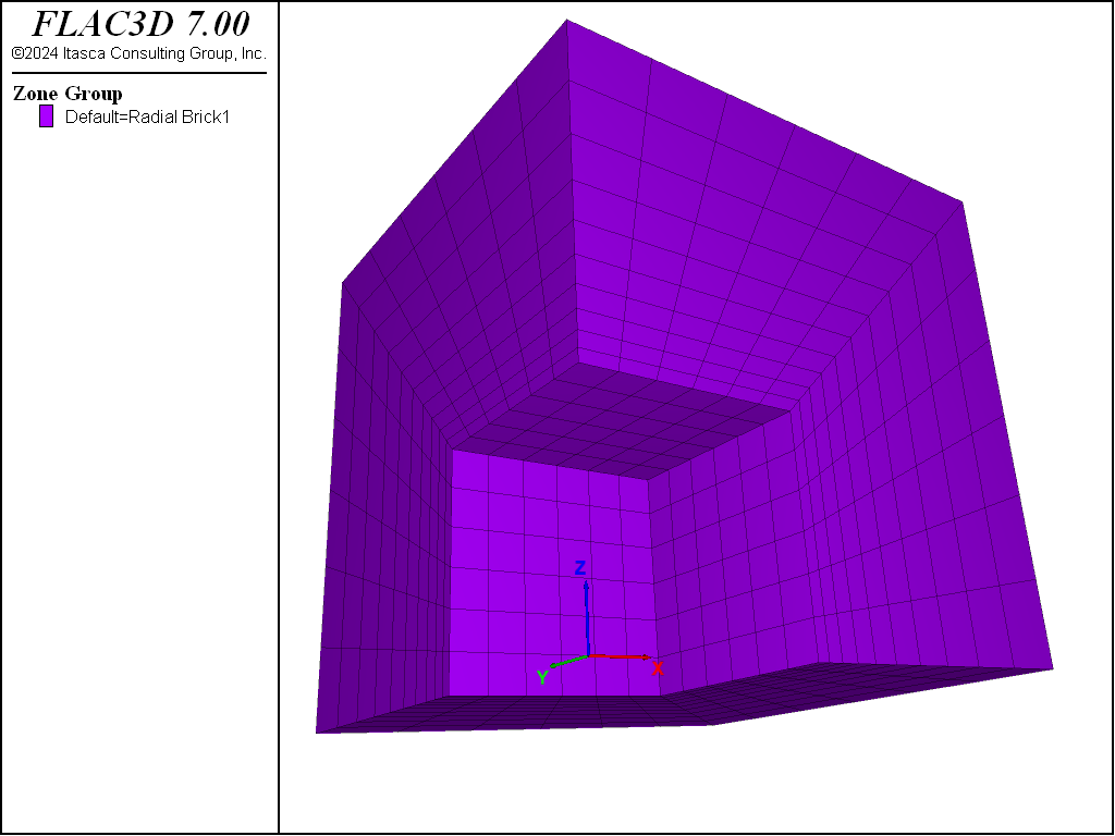
Figure 10: Initial radial-brick primitive to create a radially graded mesh around a spherical cavity.
The gridpoints within the radial brick are now relocated to form the mesh around a spherical cavity. The FISH function make_sphere loops through all the gridpoints and remaps their coordinates using a linear interpolation along radial lines from the sphere origin to the gridpoints along the outer box sides. The next example shows the make_sphere FISH function, and the figure following shows the final grid.
FISH function to position gridpoints for a mesh around a spherical shape
fish define make_sphere
    ; Loop over all GPs and remap their coordinates:
    ;  assume len>rad
    loop foreach local gp gp.list
        local p = gp.pos(gp) ; Get gp coordinate: p
        local dist = math.mag(p)
        if dist>0 then
            local k = rad/dist
            local a = p * k ; Compute a=point on sphere radially "below" p.
            local maxp = math.max(p->x,p->y,p->z)
            k = len/maxp
            local b = p * k ; Compute b=point on outer box boundary
                            ; radially "above" p.
            local u = (maxp-rad)/(len-rad) ; Linear interpolation: P=A+u*(B-A)
            gp.pos(gp) = a + (b-a)*u
        end_if
    end_loop
end
program return
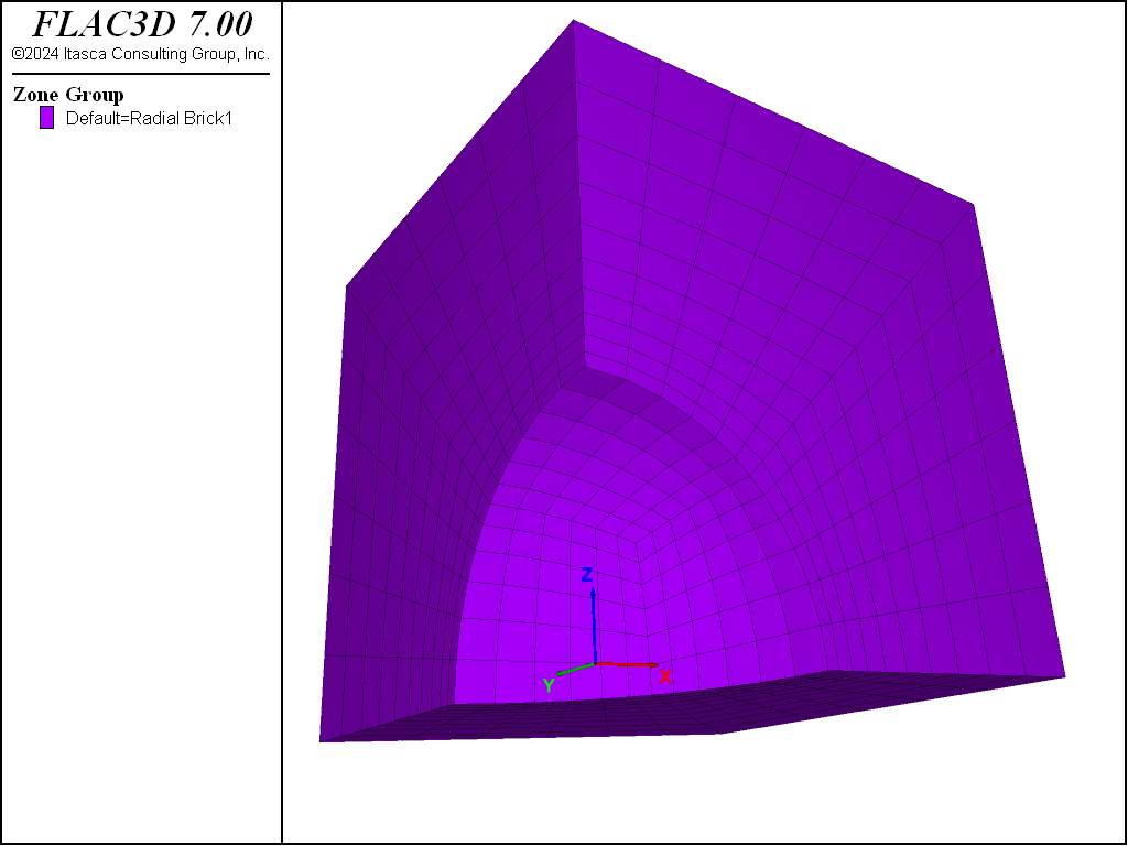
Figure 11: Radially graded mesh around a spherical cavity.
Extrusion-Based Grids
The \(i\) Extrusion pane provides a facility for creating grids based on two-dimensional geometries that are extruded (linearly extended) in the third dimension.
When working with an extrusion in the \(i\) Extrusion pane, all actions that change the state of the model are emitted as commands. These commands are echoed in the \(i\) Console pane, and they are recorded in the \(i\) State Record pane. It is possible and sometimes preferable to create zones entirely from the \(i\) Extrusion pane and start the next stage of modeling with a save file instead of creating a data file. The commands used to create the geometric model state are always stored with the save file. However, it is often advantageous to work with a data file instead, as this is a much smaller and more convenient way to recreate the geometry if necessary. The \(i\) State Record pane may be used to export all the commands that have been used to create an extrusion to a data file. These commands are documented in the Extrude section.
Use of the tools provided in the \(i\) Extrusion pane are described in detail in the \(i\) Extrusion pane section of this documentation. The following material provides a narrative overview how it is used to create grids.
Create a Set
To start an extrusion, a new set must be created in the Extrusion Pane (the pane, if not visible, is accessed via the main menu: ). Multiple extrusion sets may be defined. The “Extrusions” selector on the toolbar is used to switch between defined sets. Only one set may be active at a time.
Define the 2D Geometry
There are two view modes in the Extrusion pane: the “Construction” view (  ), and the “Extrusion” view (
  ). The former is used to define the 2D geometry. The latter is used to define the linear extrusion and is described in the next section below.
The 2D geometry is defined by drawing points and edges between points. Points may be defined by coordinates or may be defined “freehand.” Edges may be linear, curved, or arced. Curves may be arbitrarily shaped using control points. A curve may contain as many control points as needed. Further refinement is available along edges using a splitting tool.
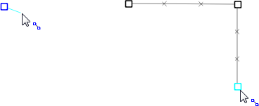
Figure 12: Points (left) and edges (right) are defined. “Exes” along the edges preview zoning. When an edge is drawn, it is initially assigned three zones by default.
When sets of edges are assembled into triangular or quadrilateral shapes, they may be defined as blocks. Once “blocked”, a given shape may be (re)zoned or grouped. When the extrusion is built into a grid in FLAC3D, only those parts of the extrusion set that have been blocked will create zones.
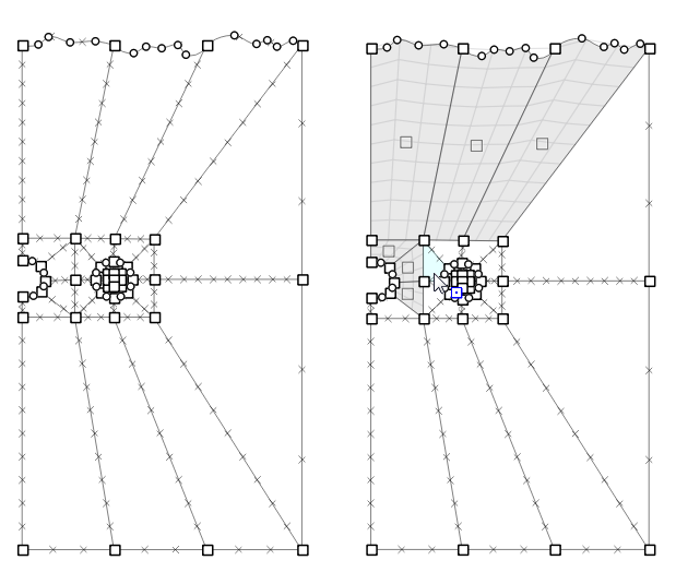
Figure 13: A set of points and edges are assembled into a quadrilateral or triangular shapes (left); they are then interactively turned into blocks (right).
Zoning and Other Operations
Zoning is set along edges by specifying the number of desired zones on that edge. Zone settings will propagate across the model as needed. A multiplier can be applied to blocks to increase zoning by an integer-factor.
In addition, there is an autozone facility available that can zone all blocks in the 2D geometry at once by defining a uniform zone length, a number of zones desired across the largest extent of the geometry, or a total number of zones within the geometry.
Groups: It is possible to select one or more points, edges, or blocks in the “Construction” view and assign them to a group and assign groups to segments and nodes in the “Extrusion” view. When this is done, any zone that is generated from the grouped points, edges, or blocks will be assigned to a zone group with the given name. Groups assigned in the “Construction” view will be in slot “Construction”, and groups assigned in the “Extrusion” view will be in slot “Extrusion”. In addition, the zones from every block will be automatically assigned a unique name in the “Block” slot, and every segment in the “Extrusion” view will be assigned a unique name in the “Segment” slot.
Splitting: The split tool can be used to split edges or blocks. When a split operation occurs, the split will propagate across all existing edges and blocks as needed.
Tracing: Bitmap or vector (DXF) images may be imported, sized, and oriented and used as “trace” guides for construction of the 2D geometry. In the latter case, a DXF will retain its “object-ness,” so it can be snapped-to when constructing points and edges for the extrusion.
Define the Extrusion
Once the 2D geometry is drawn and blocked, the extrusion is finished by switching to the “Extrusion” view to define the extent and the partitioning (blocking) of the extrusion. This is a 1D operation; the user assigns points to a horizontal line to indicate blocks, and then the segments of the line are used to define the zoning that will occur within the block represented by that segment.
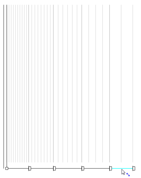
Figure 14: The extent of the extrusion and partitioning it into zoned blocks is performed in the “Extrusion” view.
When the third dimension is fully specified, zones are created from the extrusion set. Alternatively, the user may choose to export the extrusion set’s collection of 3D blocks to a new Building Blocks set in the Building Blocks Pane (see the Building Blocks-Based Grids topic next), where, presumably, further editing and refinement may occur prior to generating zones from the set.
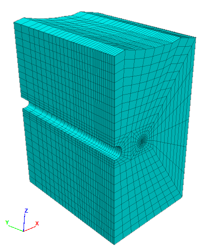
Figure 15: Zones created from the extrusion set.
Compare the image above to the final grid shown in the example of creating a grid for two tunnels with the same invert elevation. Observe that the resulting grids are comparable, but here a topography has been added to the top of the extrusion and the zoning has been graded in the direction of extrusion.
Building Blocks-Based Grids
The Building Blocks Pane provides a facility for creating grids based on three-dimensional “building blocks” that are fitted together and then zoned.
When working with an extrusion in the \(i\) Building Blocks pane, all actions that change the state of the model are emitted as commands. These commands are echoed in the \(i\) Console pane, and they are recorded in the \(i\) State Record pane. It is possible and sometimes preferable to create zones entirely from the \(i\) Building Blocks pane and start the next stage of modeling with a save file instead of creating a data file. The commands used to create the geometric model state are always stored with the save file. However, it is often advantageous to work with a data file instead, as this is a much smaller and more convenient way to recreate the geometry if necessary. The \(i\) State Record pane may be used to export all the commands that have been used to create an extrusion to a data file. These commands are documented in the Extrude section.
Use of the tools provided in the \(i\) Building Blocks pane are described in detail in the \(i\) Building Blocks section of this documentation. The following material provides a narrative overview of how it is used to create grids.
Create a Building Blocks Set
To start with building blocks, a new set must be created in the Building Blocks Pane (the pane, if not visible, is accessed via the main menu: ). Multiple sets may be defined. You can click anywhere in the blank area of the pane to create the initial set. The Sets of Blocks selector on the toolbar is used to switch between defined sets. Only one set may be active at a time.
Snap Blocks Together
On initiation of a new set, a single block is provided (assuming the box was checked in the previous dialog). The set may be developed by adding blocks using the Add Blocks tool (  ), which is done by selecting the face on an existing block to which a block should be added, then choosing the block-type to be added by rotating the mouse wheel. A quadrilateral face may have a hexahedral “brick” block type added to it, or a “wedge” type in one of two orientations. A triangular face may have a “wedge” or a “tetrahedron” block added to it.
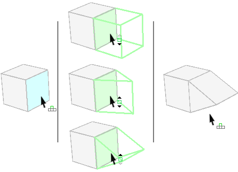
Figure 16: Left: use the “Add Blocks” tool to select a face on an existing block; center: use the mouse wheel to scroll through the options of block type to add; right: click on the desired “proto-block” to set that block in place.
Blocks are composed of points (vertices), edges, and faces. Manipulations on blocks may be performed on the whole block, or on its constituent parts. On creation, a block is given a default zoning of three zones per edge.
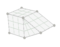
Figure 17: In base “selection” mode, the components of the block (faces, edges, points) are shown. Zoning of the block is indicated by the gray-filled grid shown on faces.
Blocks or their parts, individually or in like groups, may be moved, resized, rotated as needed and as sensible (for instance, a group of points cannot be resized as points do not have a size, though they may be moved or rotated; a single point, similarly, cannot be rotated). A screen control allows these manipulations to be performed by hand; alternatively, individual properties (position, rotation, etc.) may be specified on selected object(s) in the Control Panel.
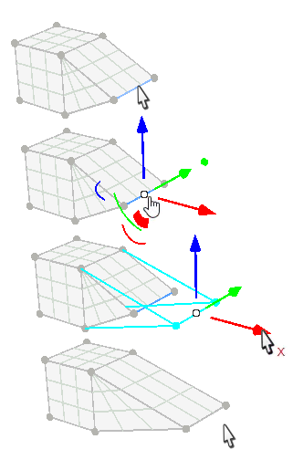
Figure 18: Selecting and moving an edge of a block.
Though there are many more facilities available in the Building Blocks Pane (described in the sections that follow below), at its simplest, an entire grid can be constructed following just the steps above. When the geometry shape is complete and zoning is set as needed, pressing the “Generate Zones” button (  ) in the Building Blocks pane will cause the zones to be generated and rendered in the Model pane.
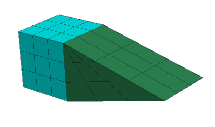
Figure 19: Zones generated from a building blocks set. Note that zones in each block from the building blocks set are automatically grouped together by block (as indicated by the coloring of the zones here).
Refinement Operations and Utilities
The simplistic illustrations above demonstrate the underlying concepts behind the Building Blocks facility. Additional tools and operations allow for significantly greater complexity to be achieved when constructing building-blocks-based grids, some of which include the following:
- Import of CAD data (DXF, STL, etc.) allows construction (tracing, as it were) of a building blocks set that is fitted to the existing 3D geometry.
- CAD data are objects that support point-snapping, which facilitates shaping blocks to fit the imported geometry.
- Edges may be split; splits will propagate automatically across existing blocks.
- Edges may be curved to fit any shape with the addition of control points.
- Blocks may be hidden/shown as needed.
- Blocks may be copied and pasted.
- Unattached blocks may be snapped to each other by matching like faces.
- A group of selected blocks comprising a layer may be duplicated and assigned a varying thickness.
- Properties of objects may be set/altered interactively or specified exactly through the Control Panel.
- The orientation of zones on a triangular face may be “cycled”.
- Like objects may be grouped together; zones derived from these objects will retain that group assignment on generation.
- Multiple forms of control are available for zoning (see the next topic below).
- A library of pre-built existing shapes and geometries is available.
As mentioned above, the present topic is only intended to offer a narrative overview of Building Blocks capabilities. See the Building Blocks Pane topics for details and instructions for using the capabilities listed above.
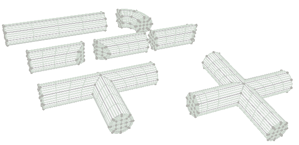
Figure 20: The “Cylinder Parts” blocks from the pre-built blocks library.
Zoning
Zoning is set along a block edge. A “Zones” attribute indicates how many zones should exist along the edge. A ratio or factor can be used to set finer sizing of zones toward the end of the edge where smaller zone sizes are needed. A block may be set to accept a multiplier, which will increase any existing zones within the block by the factor supplied. An auto-zoning facility allows for setting the zoning for an entire building-blocks set at once. Options for auto-zoning are: set a uniform zone size throughout; specify a number of zones to be used across the largest dimension of the model; or specify a total number of zones in the set.
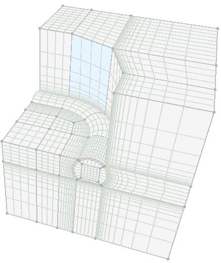
Figure 21: The “Cylinder Tunnel with Wall 90 Degree Turn” pre-built blocks. Ratios have been used to increase zone refinement around the tunnel. Blocks above the tunnel have been hidden to allow access to/visibility of the interior of the block set.
Grids from Outside FLAC3D
In addition to the built-in methods of mesh generation, meshing created by third-party applications outside FLAC3D can be imported. Currently, FLAC3D supports direct import of three different file formats:
- FLAC3D grid files (*.f3grid)
- ANSYS files (*.lis) (Note that files in this format normally come in pairs: a node file that is loaded first followed by an element file.)
- ABAQUS files (*.inp)
FLAC3D grid files is a format developed by Itasca, that has two primary benefits from the other formats:
- It exports and preserves metadata, meaning group and extra variable assignments to zones, faces, and gridpoints.
- It has a binary version, resulting in smaller files that are faster to import.
These files can be imported into a FLAC3D model by using the zone import command, by using the entry in the main menu, or in the specific case of *.f3grid files by selecting the file in the Open into Project dialog.
Once imported, the file should appear as an entry in the “Data Files” section of the \(i\) Project pane and will be added to any bundle made to archive or communicate the project.
Either the ANSYS or ABAQUS file formats (or both) are available as export options from almost all third-party meshing programs. If you have access to an advanced mesh generation, or just have a preference due to experience, you can continue to use these tools for creating FLAC3D models. Some examples include:
Itasca offers a powerful mesh generation tool that works with the popular CAD program Rhino. This tool is called Griddle, and a brief overview of it can be found in Grids from Rhino/Griddle.
Grids from Rhino/Griddle
Rhinoceros (Rhino) is a NURBS-based curves and surface representation CAD package that can be used to create closed volumes composed of meshed surfaces in 3D.[1] Griddle is Itasca’s powerful automatic grid generator that creates all-tetrahedral or hex-dominant unstructured meshes for use in FLAC3D or 3DEC. These tools are sold together but separately from FLAC3D. They represent the most advanced approach to creating complex meshes for FLAC3D. When the grid needed for a FLAC3D model exceeds the built-in capabilities provided with FLAC3D, these tools should be considered. This topic provides a brief introduction to FLAC3D users who may need to give such consideration.
The workflow for creating a complex mesh with Rhino/Griddle is straightforward. First, the model geometry is built or imported into Rhino. Next, Rhino’s surface meshing is applied. Griddle is then used to automatically remesh the surfaces to the desired density and type (triangles, quadrilaterals). The Griddle volume mesher is then called to fill the geometry with zones (all-tetrahedral or hex-dominant). The workflow is illustrated as follows.
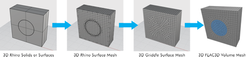
Figure 22: From left to right: an initial volume is described in Rhino; surfaces are given an initial mesh with Rhino’s own meshing tools; Griddle is used to remesh the surfaces according to user specifications; the remeshed surfaces are the basis for zoning the volume, which is then imported into FLAC3D.
All-hexahedral meshes are generally preferable for producing high-quality numeric solutions. However, the ability to produce hex-dominant meshes—that is, meshes composed mostly of hexahedral elements but also wedge, pyramid, and tetrahedral elements where necessary to conform to the geometry—with Rhino/Griddle can be a preferable trade-off when it radically reduces the challenges posed by grid complexity.
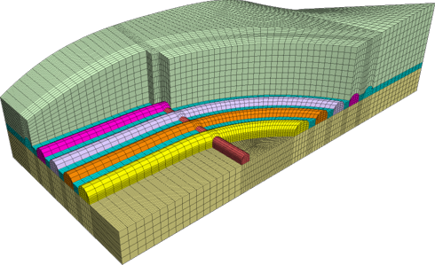
Consider the following two meshes. The first is all-hexahedral. In order to produce it, the base geometry has to be broken down (blocked) into hexahedral, tetrahedral, and prism solids. This step is time-consuming. Overall mesh generation time for this case was five hours.
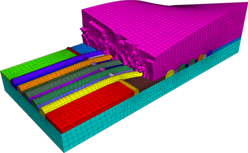
The second mesh is hex-dominant. Using Griddle, just the bounding surfaces of the tunnels and the soil layers are used as input; decomposing the model to simple primitive shapes is not required. Consequently, the total mesh generation time for this mesh was less than one hour.
Grid Generation: Additional Facilities
These additional mesh creation facilities have one thing in common: they rely on an existing mesh as a starting point for further modifications. Thus, they can be used in combination with any of the other forms of mesh generation.
The Densify operation subdivides zones into multiple zones, allowing the user to more finely discretize a coarse mesh in an area of particular interest.
Combining Geometry-based filtering with Densification can produce Octree meshes.
Finally, new zones can be extruded from an existing zone surface to an irregular geometric surface. This can be used to create complex layering (as long as the layers do not intersect) or irregular surface topography. See Surface Topography and Layering.
Densifying Grids
A simple grid is generated and then densified using the zone densify command.
New zones and faces created in this manner copy group assignments and extra variable values held
by the original, but lose all material model, stress, and other state information.
Note
Zone densification can also be done interactively from inside the Model Pane. With a set of zones selected, select the “Densify” (  ) option in the list of operations.
Figure 25: Original grid.
The following example shows commands to densify a simple grid by dividing two segments on each edge of existing zones. The above image shows the original grid; the figure following the example shows the densified grid.
Densify a grid by dividing at each edge of the original zones
model new
model large-strain off
zone create wedge size 4 4 4
plot 'Wedge' export bitmap filename 'densify1.png'
;
zone densify segments 2
plot 'Wedge' export bitmap filename 'densify2.png'

Figure 26: Densified grid by dividing segments on each edge of zones.
In addition to dividing segments, maximum length of the refining zones can be specified with the edge-limit keyword. No matter how edge-limit or segments is used, FLAC3D always densifies the grid by dividing the zone edges with a segment number of an integer. The next example shows how to densify a grid in the range of \(z\)-coordinates between 2 and 4 by setting the edge limit to be 0.5.
Densify a grid by specifying the edge limit length
model new
model large-strain off
zone create brick size 4 4 4
plot 'Brick' export bitmap filename 'densify3.png'
;
zone densify edge-limit 0.5 range position-z 2 4
zone attach by-face
;
plot 'Brick' export bitmap filename 'densify4.png'

Figure 27: Original grid.
The zone attach by-face command in this example is used to attach faces of sub-grids together rigidly to form a single grid. Always use the zone attach by-face command after the zone densify command if there are different numbers of gridpoints along faces of different zones. The image above is the original grid for this example; the image below is the densified grid.
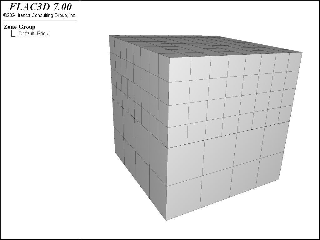
Figure 28: Densified grid by setting maximum lengths.
Sometimes geometric data contained in geometric sets defines the space where densification is needed. The next example presents a method to densify a space between two geometric sets. See Working with Geometric Data for a general overview and description of using geometric data to identify objects in the model.
In this example, each geometric set is defined by two polygons. The zone densify command uses a geometry range element that selects any zones with a centroid such that a ray with direction of (0,0,1) will intersect once with any of the polygons making up setA or setB. See the range geometry-space documentation for details.
The zone attach by-face command here is used to attach faces of sub-grids together rigidly to form a single grid for all zones. The next two figures plot the original and densified grids.
Densify a grid using geometric information
model new
model large-strain off
zone create brick size 10 10 10
;
geometry set "setA" polygon create by-positions (0,0,1) (5,0,1)   ...
                                                (5,10,1) (0,10,1)
geometry set "setA" polygon create by-positions (5,0,1) (10,0,5)  ...
                                                (10,10,5) (5,10,1)
geometry set "setB" polygon create by-positions (0,0,5) (5,0,5)   ...
                                                (5,10,5) (0,10,5)
geometry set "setB" polygon create by-positions (5,0,5) (10,0,10) ...
                                                (10,10,10) (5,10,5)
plot 'Brick2' export bitmap filename 'densify5.png'

zone densify segments 2 range geometry-space "setA" set "setB" count 1
zone attach by-face
;
plot 'Brick2' export bitmap filename 'densify6.png'

Figure 29: Original grid.
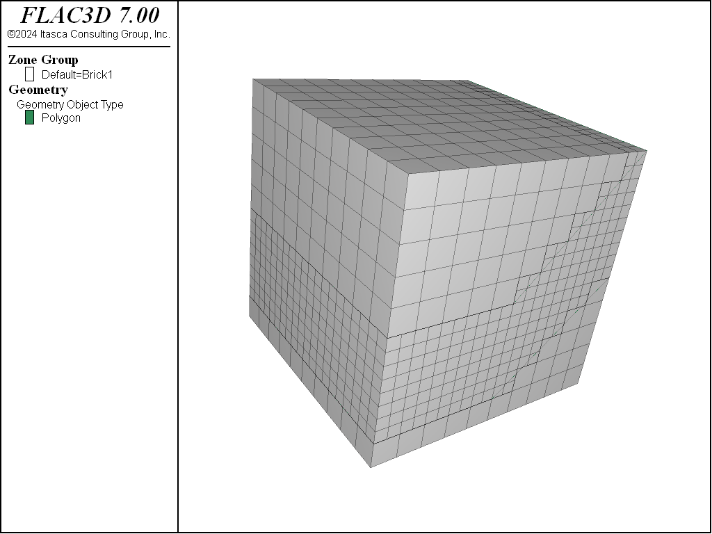
Figure 30: Densified grid using geometric data.
Geometry-Based Densification: Octree Meshing
Grid densification based on geometric data in geometric sets is often used to approximate material property changes on a very irregular boundary, when exact conformation to the surface is not important physically. Often orebody and other kinds of geologic structures fall into this category.
The command zone densify can be used to subdivide zones selected by their proximity to a geometry surface. Using it in combination with the range geometry-distance range element and using the repeat keyword allows the creation of an octtree mesh in a single command.
For example, the command
zone densify segments 2 gradient-limit edge-limit 0.05 ...
            repeat range geometry-distance 'intcylinder' gap 0.0 extent
can be used to generate an octree mesh based on proximity to the “intcylinder” geometry set.
It is important to be clear about what each of the keywords invoked above is doing.
- The segments keyword indicates that each level of densification will subdivide a zone by 2 in each direction, resulting in eight new zones for every original.
- The gradient-limit keyword affects the zones tagged for densification. It ensures that the maximum difference in zone size from one zone to the next is one level of densification.
- The edge-limit keyword, in combination with the repeat described below, indicates that zones will be tagged for densification if they have an edge length longer than 0.05.
- The repeat keyword indicates that a single densification pass will be made over the zones, then if any zones were densified, a +new+ list of zones will be selected for densification. This operation will be repeated until no zones are left to be densified, either because they do not fall within the range or because they are already smaller than the edge-limit specified.
- The
range geometry-distanceselects zones that fall within a gap distance from the intcylinder geometry set. Since the gap is zero in this case, it selects zones that actually intersect the surface. - The extent keyword indicates that the distance from the surface should be judged by the +Cartesian extent+ of the zone, rather than just the zone centroid. If this was not used, a non-zero gap would be required for there to be any chance of a zone falling within the range.
The results of this command are shown here.
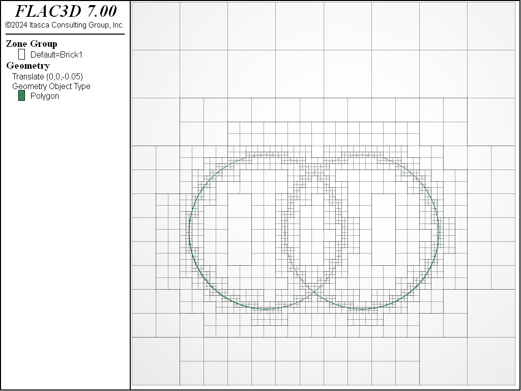
Figure 31: Octree mesh generated with zone densify.
Remember that this mesh should not be run until the zone attach by-face command is used to attach hanging nodes to adjacent faces. Also note that large gradients in zone size can increase the time it takes to reach equilibrium and change the path the model takes to get there.
For a more realistic example, the following data file takes a simple rectangular mesh and uses it as a starting point to create an octree mesh of a complex orebody.
model new
zone create brick size (10,15,10) point 0 (25000,20000,0) ...
                                  point 1 (35000,20000,0) ...
                                  point 2 (25000,35000,0) ...
                                  point 3 (25000,20000,10000)
geometry import 'orebody.stl'
zone densify segments 2 gradient-limit edge-limit 50 repeat ...
             range geometry-distance 'orebody' gap 0.0 extent
zone group 'orebody' range geometry-space 'orebody' count odd
The result of that operation is shown in the figure below. The last zone group command uses the range geometry-space range element to select zones “inside” the geometric surface.
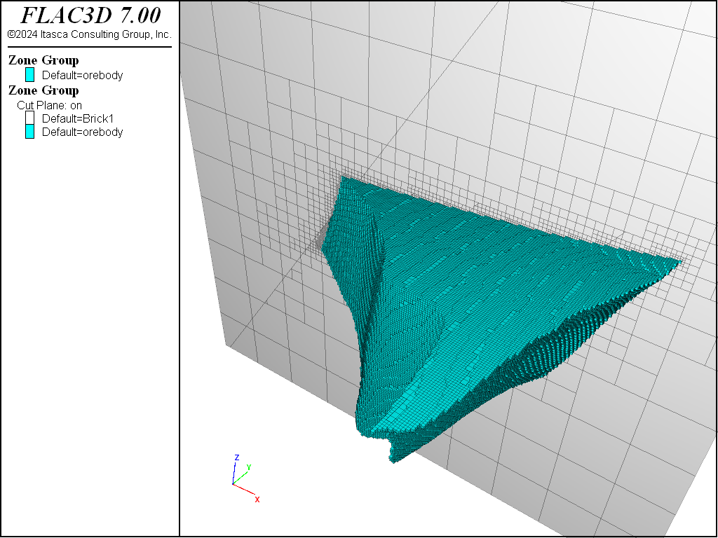
Figure 32: Octree mesh generated with zone densify.
Surface Topography and Layering
FLAC3D provides a zone generate from-topography command to generate a grid between the surface faces of an existing grid and a geometry set that characterizes the topography. The zones are created by extruding from faces in a specified range along a ray direction to a specified geometry set. This can be used to create a series of irregular non-intersecting layers, or most commonly, to add a layer of zones to the top that conforms to an irregular topographic surface. Some simple examples of its use follows.
To create a grid that conforms to a topographic surface, a geometry set must be specified. The easiest way to create a geometry set is via the geometry import command. Additional commands are available for manipulation of edges, polygons, and nodes, as well as other operations on geometric sets in their entireties.
An initial grid must exist before using the zone generate from-topography command. Only the zone faces satisfying all of the following criteria will be selected:
- The faces must be in the range.
- The faces must be on the existing grid surface, and any interior faces will be neglected.
- The outward normal vector of the faces must make an angle with the ray of less than 89.427 degrees. This will exclude the faces parallel to the ray (with a crossing angle of 90 degrees) or the faces facing a relatively opposite direction of the ray (with a crossing angle greater than 90 but not greater than 180 degrees).
The data file in the next example first imports geometry data from the STL format file surface1.stl and places it into a geometry set called surface1. (By default, the geometry set name is the same as the file name just imported.) The data file then creates a background grid with a group name Layer1. The geometry set and the background grid are shown in the next image below. It can be seen that if projected to the \(x\)-\(y\) plane, the geometry set will fully cover the background grid, so any node in a valid face in the range will have an intersection point with the geometry set if extruding along the ray direction.
Create a grid and a geometric set
model new
geometry import 'surface1.stl'
zone create brick size 50 40 5 ...
                  point 0 (0,    0,-4000) point 1 (15000,0,-4000) ...
                  point 2 (0,12000,-4000) point 3 (    0,0,-2000) ...
                  group 'Layer1'
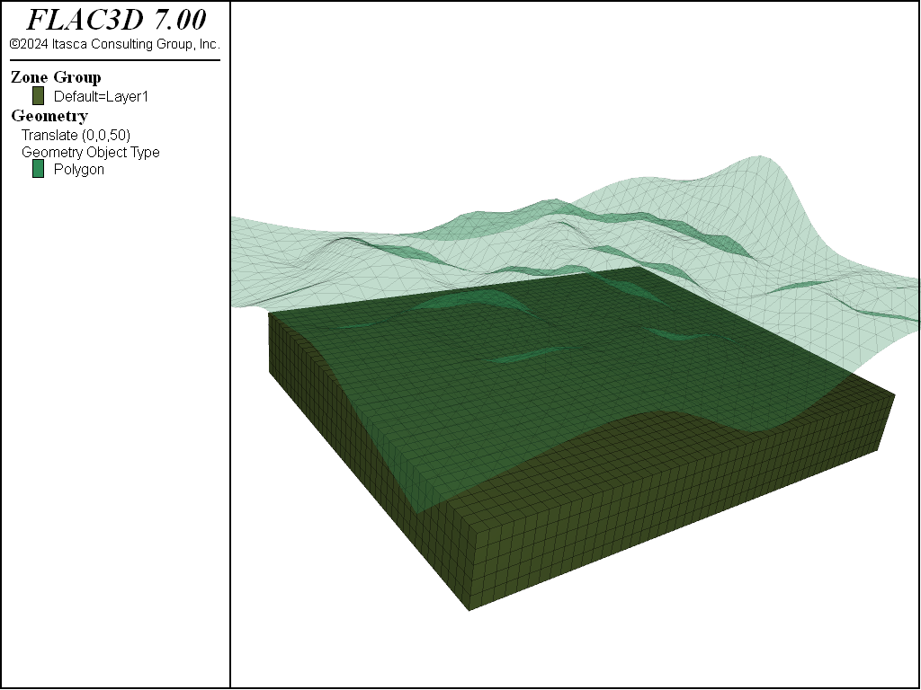
Figure 33: The existing grid and the geometry set.
Next the zone generate from-topography command is added. In the command, the surface1 geometry set is specified. No ray direction is specified, so the default direction (0, 0, 1) is used by default. The segment number is 8, so 8 zones will be created between the selected faces and the geometric surface. The newly created zones will be assigned the group name Layer2 in slot Default. No range is assigned to the faces in this command, so all faces on the existing grid (group Layer1 ) surfaces are subjected to extrusion to the geometry set. However, the zone faces on the four side surfaces whose normal vector is vertical to the ray direction (0, 0, 1), and the faces on the bottom whose normal vector is in the opposite direction of the ray (with a crossing angle of 180 degrees), are neglected in this example, so only the faces on the top surface of group Layer1 will actually be used to create the new grid. The completed grid is shown in the next figure. The topography of the geometry set is correctly featured in the grid.
Add surface topography zones
model new
geometry import 'surface1.stl'
zone create brick size 50 40 5 ...
                  point 0 (0,    0,-4000) point 1 (15000,0,-4000) ...
                  point 2 (0,12000,-4000) point 3 (    0,0,-2000) ...
                  group 'Layer1'
zone generate from-topography geometry-set 'surface1' ...
                              segments 8 group 'Layer2'
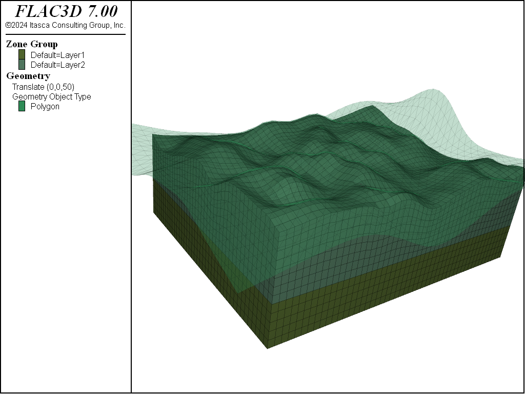
Figure 34: Grid created by the zone generate from-topography command.
The next example adds two new keywords to the zone generate from-topography command. The first is ratio, which is set to 0.6. This changes the distribution of zone sizes as you approach the surface; in this case each zone is 0.6 time the size of the next. The second is face-group, which assigns a group name to the new zone surface created for ease of reference later.
Grade zones toward surface
model new
geometry import 'surface1.stl'
zone create brick size 50 40 5 ...
                  point 0 (0,    0,-4000) point 1 (15000,0,-4000) ...
                  point 2 (0,12000,-4000) point 3 (    0,0,-2000) ...
                  group 'Layer1'
zone generate from-topography geometry-set 'surface1' ...
                              segments 8 ratio 0.6 group 'Layer2' ...
                              face-group 'Surface'
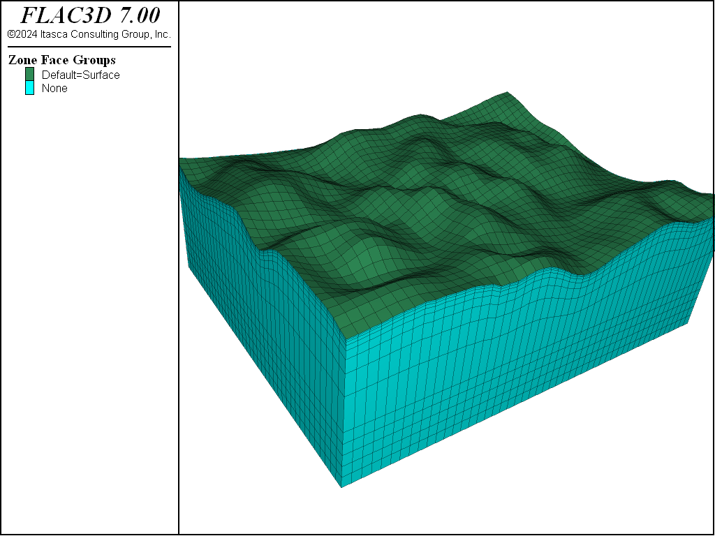
Figure 35: Grid created by the zone generate from-topography command (ratio=0.6).
In the next example, a range is applied to the faces on the background grid. This range is limited to only the faces whose centroid coordinates fall in the ranges 0 ≤ \(x\) ≤ 5000 and 0 ≤ \(y\) ≤ 50000. It should be emphasized that the range in zone generate from-topography is selecting zone faces.
Limit area of surface
model new
geometry import 'surface1.stl'
zone create brick size 50 40 5 ...
                  point 0 (0,    0,-4000) point 1 (15000,0,-4000) ...
                  point 2 (0,12000,-4000) point 3 (    0,0,-2000) ...
                  group 'Layer1'
zone generate from-topography geometry-set 'surface1' ...
                              segments 8 ratio 0.6 group 'Layer2' ...
                              range position-x 0 5000 position-y 0 5000
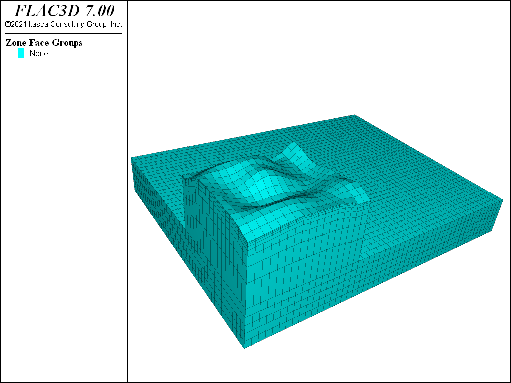
Figure 36: Grid created by the zone generate from-topography command (with a range applied to the faces).
In some cases, the geometric surface may not cover the projected area of the selected faces in the ray direction. To deal with this case, FLAC3D will first find a point A in the geometry set that is closest to the ray that starts at the relevant gridpoint, and then find a “virtual” intersection point B so that points A and B have the same distance to the projected plane. The completed grid is shown in the second figure below.
Surface that does not cover zone extent
model new
geometry import 'surface1.stl'
zone create brick size 50 40 5 ...
            point 0 (-10000,-10000,-4000) point 1 ( 15000,-10000,-4000) ...
            point 2 (-10000, 12000,-4000) point 3 (-10000,-10000,-2000) ...
            group 'Layer1'
zone generate from-topography geometry-set 'surface1' ...
                              segments 8 ratio 0.6 group 'Layer2'
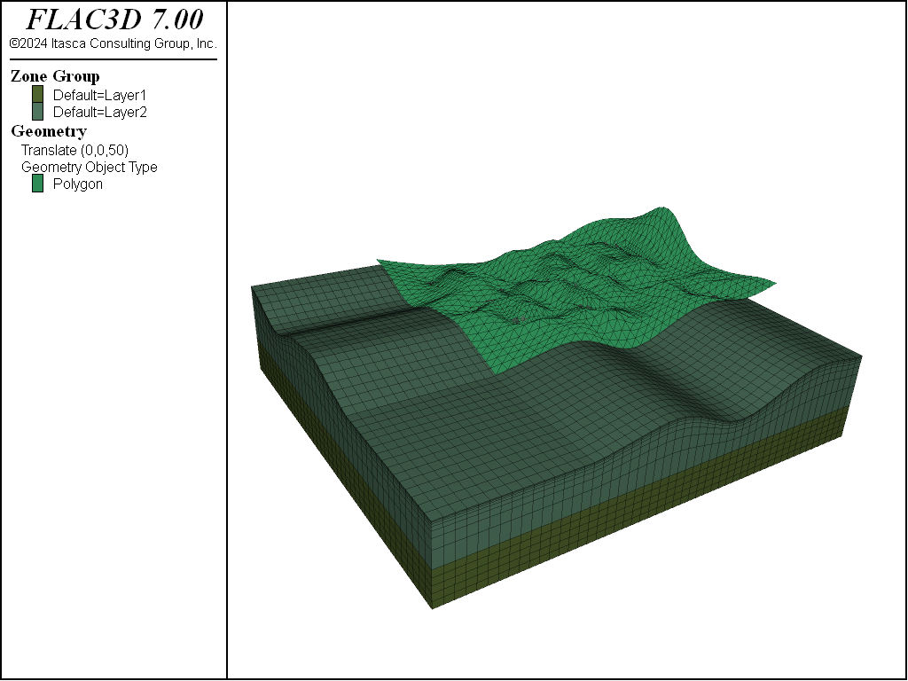
Figure 37: Grid created by the zone generate from-topography command (the geometry set does not fully cover the background grid if projected into a plane perpendicular to the ray).
The zone generate from-topography command can be used multiple times to create a grid with multiple layers. Each time the zone generate from-topography command is employed, the most updated grid will be regarded as the background grid. The zone-face keyword can also be used to mark the new zone surface faces in order to use them in the next layer.
In the next example, the second geometry set (called surface2) is created with a simple geometry set command. Then a quadrilateral polygon is created in it using geometry polygon create. Next, a second zone generate from-topography command is issued to fill the space between the irregular surface (labeled Surface) and the polygon in set surface2.
Note that the faces labeled Surface could subsequently be used to generate an interface, if desired.
Create a grid with multiple geometric sets
model new
geometry import 'surface1.stl'
zone create brick size 50 40 5 ...
                  point 0 (0,    0,-4000) point 1 (15000,0,-4000) ...
                  point 2 (0,12000,-4000) point 3 (    0,0,-2000) ...
                  group 'Layer1'
zone generate from-topography geometry-set 'surface1' ...
                              segments 8 ratio 0.8 group 'Layer2' ...
                              face-group 'Surface'
;  Create the next layer
geometry select 'surface2'
geometry polygon create by-positions (0,0,3000) (15000,0,3000) ...
                                     (15000,12000,3000) (0,12000,3000)
zone generate from-topography geometry-set 'surface2' ...
                              segments 8 ratio 1.2 group 'Layer3' ...
                              range group 'Surface'
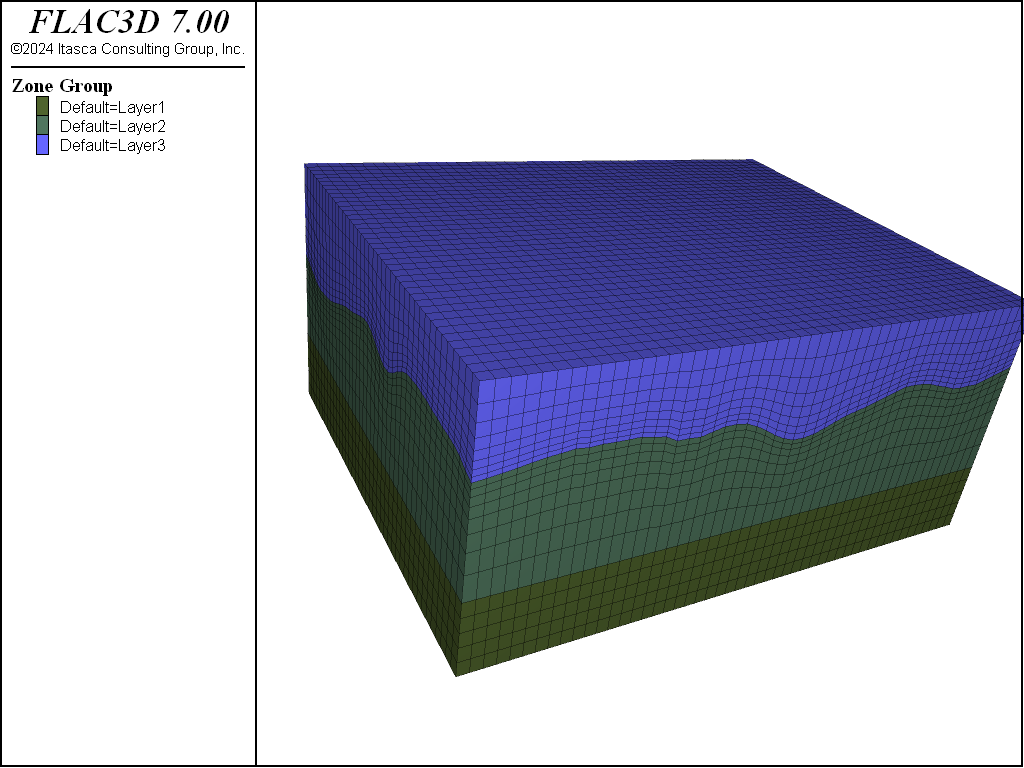
Figure 38: Grid created by multiple zone generate from-topography commands.
Endnotes
| [1] | See https://en.wikipedia.org/wiki/Rhinoceros_3D. |
| Was this helpful? ... | FLAC3D © 2019, Itasca | Updated: Feb 25, 2024 |