Kelvin Model: Oedometer Test

Note

To view this project in FLAC3D, use the menu command Help ► Examples…. Choose “Creep/OedometerKelvin” and select “OedometerKelvin.prj” to load. The project’s main data files are shown at the end of this example.

This example compares the numerical and analytical solutions of an oedometer test carried out on a generalized Kelvin substance (Kelvin cell in series with a shear spring). In the oedometer test, the base of the sample is fixed, lateral deformations are prevented, and a constant vertical load \(P\) is applied at the top of the specimen.

The analytical solution for vertical strain and stresses is

(1)\[\epsilon_{zz}=- {{P} \over {K}} b \left[ c \left( 1 - e^{-at} \right) + 1 \right]\]

(2)\[\sigma_{zz} = -P\]

(3)\[\sigma_{xx} = \sigma_{yy} = {{K} \over {2}} \left( 3 \epsilon_{zz} + {{P} \over {K}} \right)\]

where \(b\), \(a\), and \(c\) are the three constants:

(4)\[b = {{K} \over {K + 4G/3}}\]

(5)\[a = {{G_{K}/G + b} \over {\eta / G}}\]

(6)\[c = {{1 - b} \over {G_{k} / G + b}}\]

\(K\), \(G_{K}\), \(G\) are bulk and shear moduli of the substance (\(G_{k}\) is for the Kelvin cell, \(G\) is for the spring in series), and \(\eta\) is the viscosity.

The numerical simulation is carried out simultaneously on two samples, each represented by one zone, using the Burgers model and the Burgers-Mohr model.

Because no value is assigned to the property viscosity-maxwell, the Maxwell dashpot is not taken into account by the models. Also, the cohesion property is set to a high value to prevent triggering of the plasticity logic for the Burgers-Mohr model. The initial state is first obtained by cycling the model to elastic equilibrium. Velocities are then reset to zero. For the viscous response, the initial timestep is set to a small value (\(\Delta t\) = 10^-3) compared to the ratio of viscosity over shear modulus (\(\eta /G_K\) = 1.0). With the choice of creep timestep parameter settings used in the example, the timestep increases by a factor of 1.01 when the out-of-balance force ratio is less than 10^-4, until \(\Delta t\) = 0.1. At the end of the simulation, the response is for two shear moduli, \(G_{k}\) and \(G\), acting in series (long-term behavior). Figure 1 and Figure 2 show the agreement between analytical solutions and numerical predictions for stresses and strains in the two samples.

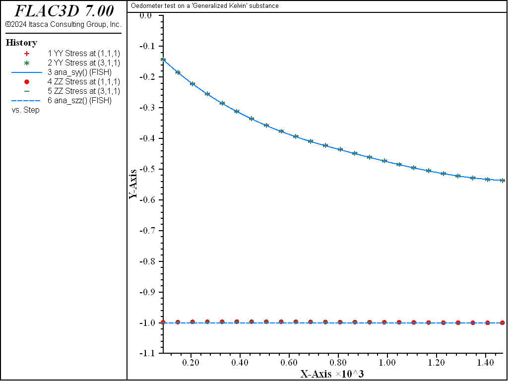
Figure 1: Oedometer test on a Kelvin substance: analytical and numerical stress values versus time.

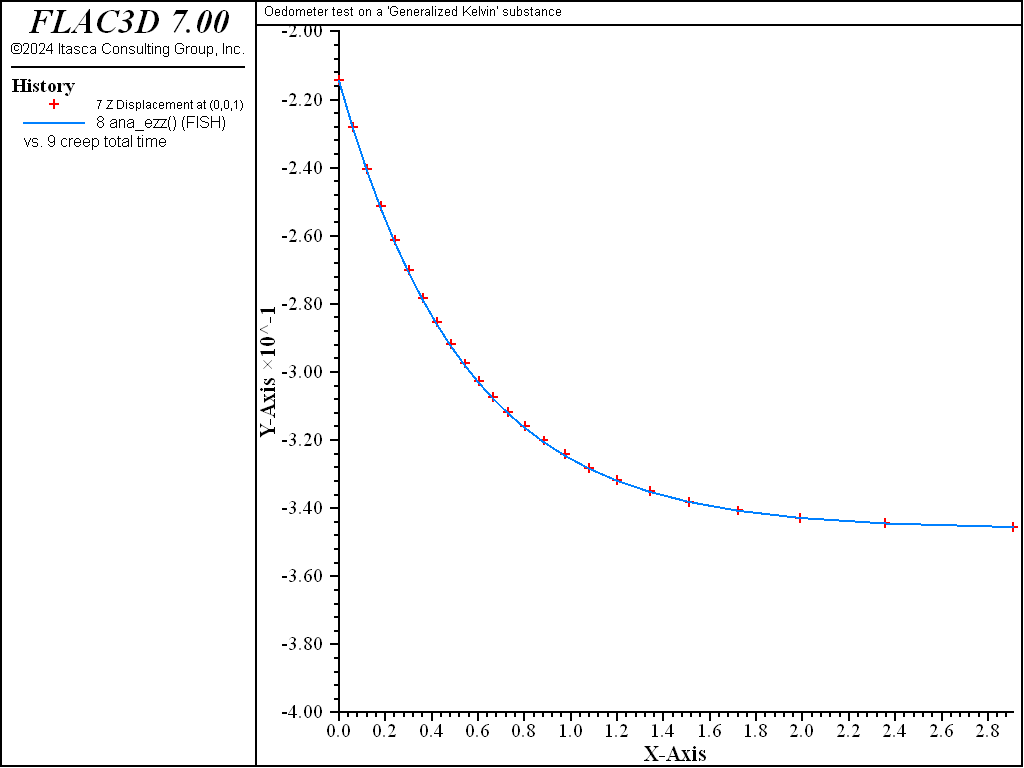
Figure 2: Oedometer test on a Kelvin substance: analytical and numerical strain values versus time.

Data File

;------------------------------------------------------------
;       Oedometer test -- Generalized Kelvin substance
;-------------------------------------------------------------------
model new
model large-strain off
fish automatic-create off
model title "Oedometer test on a 'Generalized Kelvin' substance" 
model configure creep
program call 'parameter'
[ini_cons]
; --- model ---
zone create brick size 3 1 1
zone cmodel burgers      range position-x 0 1
zone cmodel burgers-mohr range position-x 2 3
zone cmodel assign null         range position-x 1 2
;
zone property density 1 bulk [c_bu] 
zone property shear-maxwell [c_sh] shear-kelvin [c_ksh] ...
              viscosity-kelvin [c_kvi] range position-x 0 1
zone property shear-maxwell [c_sh] shear-kelvin [c_ksh] ...
              viscosity-kelvin [c_kvi] cohesion 1e20 tension 1e20 ...
              range position-x 2 3
;
zone gridpoint fix velocity-x 
zone gridpoint fix velocity-y
zone gridpoint fix velocity-z range position-z 0
zone face apply stress-normal -1.0 range position-z 1
; --- elastic equilibrium ---
model solve ratio 1e-4
; --- reset velocities to zero ---
zone gridpoint initialize velocity (0,0,0)
; --- histories ---
history interval  1
zone history stress-yy position 1 1 1
zone history stress-yy position 3 1 1
fish history ana_syy
zone history stress-zz position 1 1 1
zone history stress-zz position 3 1 1
fish history ana_szz
zone history displacement-z position 0 0 1
fish history ana_ezz
model history creep time-total
; --- viscous behaviour ---
model creep timestep starting 1.e-3
model creep timestep lower-bound=1e-4 
model creep timestep upper-bound 5e-4 
model creep timestep minimum=1.e-3 
model creep timestep maximum=0.1
model solve time-total=3.
model save 'kelvin'