Axially Loaded Pile
Problem Statement
Note
The project file for this example is available to be viewed/run in FLAC3D.[1] The main data files used are shown at the end of this example. The remaining data files can be found in the project.
Piles transfer axial loads to the ground via two mechanisms: skin friction along the shaft and end-bearing. The pile logic directly includes skin-friction effects, and end-bearing effects can be included by making a small modification to the linkage at the bottom pile node. Both effects are examined in this example.
Skin Friction — The ultimate bearing capacity of a single pile of length \(L\) in a cohesionless soil is a function of the shaft resistance due to skin friction, as given by (Cernica 1995)
| where: | \(L_i\) | = | increment \(i\) of pile length; |
| \((a_s)_i\) | = | area of pile surface in length \(\Delta L\) in contact with soil; and | |
| \((s_s)_i\) | = | unit shaft resistance. |
For uniform soil conditions and constant pile cross-section, \(s_s\) and \(a_s\) are constant and
In free-draining cohesionless soil, the value for \(s_s\) is assumed to equal
| where: | \(K_s\) | = | average coefficient of earth pressure on the pile shaft; |
| \(\sigma_{avg}\) | = | average effective overburden pressure along the pile shaft; and | |
| \(\phi_s\) | = | angle of skin friction. |
End Bearing — The ultimate bearing capacity due to end-bearing resistance of a single pile is typically calculated based on the principles of bearing capacity for shallow foundations using the bearing capacity factors \(N_c\), \(N_q\), and \(N_{\gamma}\). For a single pile in a cohesionless soil, the end-bearing capacity, \(Q_p\), is given by (Cernica 1995)
| where: | \(A_p\) | = | area of pile tip; |
| \(\gamma\) | = | unit weight of soil; | |
| \(N_q\) | = | \(\bigl ( {{1 + \sin \phi} \over {1 - \sin \phi}} \bigr )^2\); and | |
| \(\phi\) | = | the friction angle of the soil. |
The total pile capacity for a single pile in a cohesionless soil is then
In this example, a single pile in a cohesionless soil is axially loaded by applying a constant vertical velocity to the top of the pile. The axial force in the top pile element is monitored to determine the limiting load (i.e., the ultimate bearing capacity). The pile length within the soil is 7 m, and the pile diameter is 1 m. The soil has a friction angle of 10°, and the skin friction between the pile shaft and soil is also assumed to be 10°. The unit weight of the soil is 20,000 N/m3, and the stress state is assumed to be isotropic (\(K_s\) = 1). The average effective overburden pressure along the pile shaft is calculated at the mid-depth of the pile to be 70,000 Pa, assuming that the strength varies linearly.
If only skin friction along the shaft is considered, using equations (2) and (3), the ultimate bearing capacity for the pile is \(Q_s\) = 271 kN. If the end-bearing capacity is included, using equation (5), the total bearing capacity \(Q\) = 493 kN.
In the FLAC3D data file, the analysis is first conducted by only accounting for the shaft resistance. coupling-friction-shear is set to 10°, and the other coupling spring strength parameters are set to zero. The history of the axial force in the top pile element is plotted versus vertical displacement of the top node in Figure 1. The limiting load is equal to 280 kN.
This figure also contains a plot of the coupling-spring shear-stress distribution along the pile
and shows the linear increase in shear stress with depth. Note that combined damping
(structure damping combined-local), rather than local damping, is used for this analysis
because there is significant uniform motion in one direction as a result of the downward loading on
the pile (see Mechanical Damping).
The link at the bottom node provides the pile-grid interaction described in Pile Structural Elements. This interaction does not include end-bearing effects. To include end-bearing effects, we must delete this link, replace it with a new link containing a normal-yield spring in the axial direction, and specify appropriate spring properties. We include end-bearing effects by including commands after creating the pile:
struct link delete range position-z 4.0
struct link create target zone group 'End' range position-z 4.0
struct link attach x=normal-yield y=free z=free                           range group 'End'
struct link attach rotation-x=free rotation-y=free rotation-z=free        range group 'End'
struct link property x area=1.0 stiffness=5.4e11 yield-compression=2.22e5 range group 'End'
The first two commands delete the existing link and replace it with a new link that is given a
group name of End. All link properties are specified with respect to the node-local system
of the source node. Because the source node is used by a pile element, its node-local system will
be oriented such that the \(x\)-direction is aligned with the pile axis. Note that this
orientation is set automatically at the start of a set of cycles, or when the model cycle 0 command is executed.
The next three commands set attachment conditions for all link directions to be free, except for
the \(x\)-direction, in which a normal-yield spring is inserted. The final command sets the
properties of this spring as follows. The spring stiffness, \(K\), should be at least as large
as the axially directed stiffness of the bottom node in the original system (before its link has
been deleted). The command structure node list stiffness shows this value to be 5.4 × 10¹¹ N/m. Thus, we set the spring area equal to 1.0 m2, and the spring stiffness equal to 5.4 × 10¹¹ N/m3. We set the compressive yield strength of the spring equal to the bearing capacity at 7 m depth, as given by equation (4), to equal 222 kN.
The results are shown in Figure 2. The limiting load equals 490 kN when end-bearing resistance is included. Both FLAC3D results (for skin friction alone, and for skin friction plus end bearing) compare well with the solutions given in equations (2) and (5).
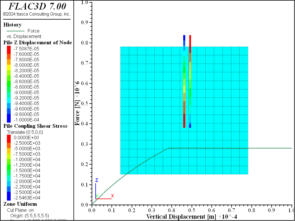
Figure 1: Friction pile: Top force-displacement history and shear stress along shaft.
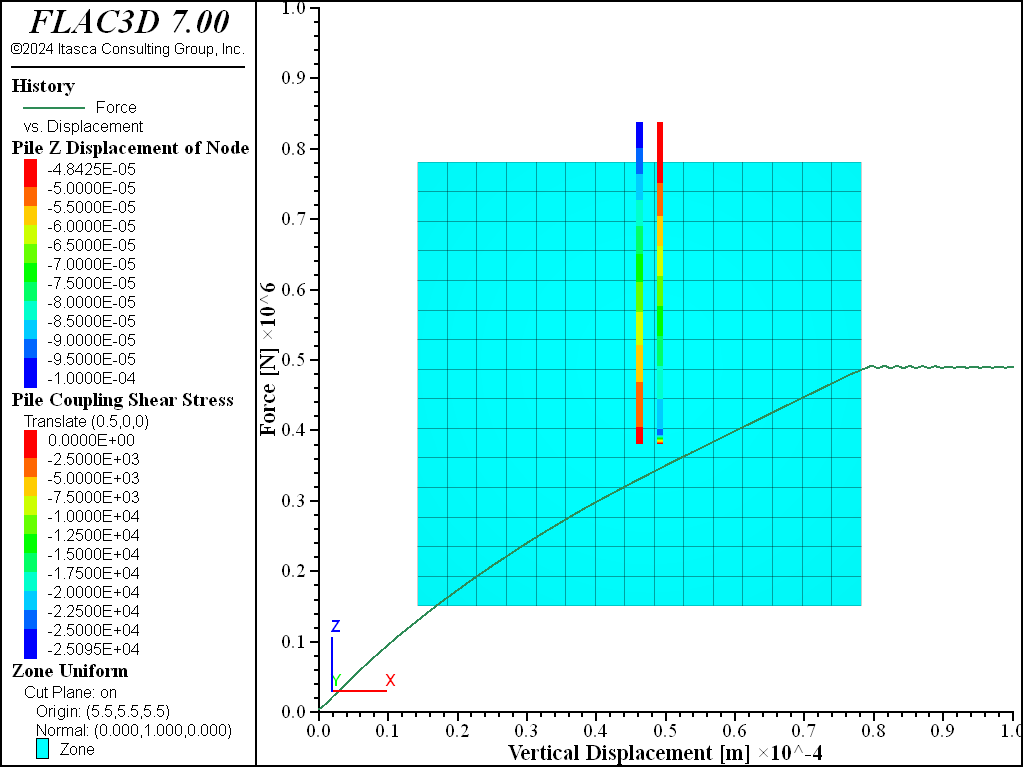
Figure 2: Friction and end-bearing pile: Top force-displacement history and shear stress along shaft.
References
Cernica, J. N. Geotechnical Engineering: Foundation Design, New York: John Wiley & Sons Inc. (1995).
Data File
AxiallyLoaded.dat
; Axially loaded pile example application
model new
model large-strain off
model title "Axially Loaded Pile"
; Create the grid
zone create brick size 15 15 15 edge=11
zone face skin ; Label model boundaries
; Assign constitutive model and propertie
zone cmodel assign elastic
zone property bulk=5e9 shear=1e9 density=2000
; Boundary conditions
zone face apply velocity-normal 0 range group 'East' or 'West'
zone face apply velocity-normal 0 range group 'North' or 'South'
zone face apply velocity-normal 0 range group 'Bottom'
; Initial conditions
model gravity 10
zone initialize-stresses
model solve ratio-local 1e-4 ; Should be instant
; =======================================================
; Create a pile in the center of the soil block
struct pile create by-line (5.5, 5.5, 12) (5.5, 5.5, 4) segments=32
struct pile property young=8.0e10 poisson=0.30 cross-sectional-area=0.7854 ...
                     moi-polar=0.0 moi-y=0.0 moi-z=0.0 perimeter=3.14 ...
                     coupling-stiffness-shear=1.3e11 ...
                     coupling-cohesion-shear=0.0 ...
                     coupling-friction-shear=10.0 ...
                     coupling-stiffness-normal=1.3e11 ...
                     coupling-cohesion-normal=0.0 ...
                     coupling-friction-normal=0.0 coupling-gap-normal=off
; =======================================================
; Specify and apply velocity to pile tip.
struct node fix velocity-x                     range position-z 12
struct node initialize velocity-x 0.5e-8 local range position-z 12
; =======================================================
; Set up histories for monitoring model behavior
struct node history name='disp'  displacement-z position (5.5,5.5,12)
struct pile history name='force' force-x position (5.5,5.5,12)
; =======================================================
struct mechanical damping combined-local
model save 'Initial'
; =======================================================
; Apply velocity to achieve total displacement of 10e-5 m
model cycle 20000
model save 'AxiallyLoaded-1'
; =======================================================
; Include end-bearing effect
model restore 'Initial'
struct link delete range position-z 4.0
struct link create target zone group 'End' range position-z 4.0
struct link attach x=normal-yield y=free z=free ...
                               range group 'End'
struct link attach rotation-x=free rotation-y=free rotation-z=free ...
                                                 range group 'End'
struct link property x area=1.0 stiffness=5.4e11 yield-compression=2.22e5 ...
                                                         range group 'End'
model cycle 20000
model save 'AxiallyLoaded-2'
Endnotes
| [1] | To view this project in FLAC3D, use the program menu.
⮡ FLAC |
| Was this helpful? ... | FLAC3D © 2019, Itasca | Updated: Feb 25, 2024 |