Generating a Bonded Assembly
Introduction
Note
The project file for this example may be viewed/run in PFC.[1] The data files used are shown at the end of this example.
PFC is capable of reproducing many behaviors observed in solid materials by using contact models that allow for the creation of bonds at contacts. Bonds conceptually represent material between pieces (i.e., balls, pebbles, and facets) that may carry loads to specified limits. If stresses are introduced below this threshold, the material may act similar to a continuum approximation of a solid. Once local strength limits are exceeded, bonds break and neighboring pieces are free to behave as if they are in an unbonded state. For instance, frictional slip may occur locally, simulating the initiation and propagation of fractures. The bulk response can be quantitatively compared with similar laboratory experiments, allowing one to calibrate the synthetic material. The bonded-particle modeling methodology is discussed thoroughly in [Potyondy2015a].
A simple material is created in this tutorial using the linear parallel bond model. The contact properties are specified directly, and the specimen is equilibrated.
Numerical Model
The first step of any PFC model is to select the size of the simulation domain. By definition, the domain is an axis-aligned box within which all model components exist. This command sets the domain extent to be a cubic box with side length of 20.0 units centered on the origin of the model (always at (0.0,0.0,0.0)). This is achieved by specifying the edges of the extent in the \(x\)-direction only. If the extent edges in the \(y\)- and/or \(z\)-direction(s) are not specified, then the extent edges of the preceding direction are used.
model domain extent -10 10
The next step is to explicitly specify the default contact models with the Contact Model Assignment Table (CMAT). This is an important and mandatory step of the PFC modeling procedure. In this model, two types of contacts will be present: ball-ball and ball-facet contacts. We will use the linear contact model for ball-facet contacts. To generate a bonded specimen, we will use the linear parallel bond model for ball-ball contacts. Also note the use of the proximity keyword; it ensures that all contacts will be created between pieces if their surfaces are within the specified gap.
contact cmat proximity 0.1
contact cmat default model linear property kn 1e6
contact cmat default type ball-ball model linearpbond property kn 1e6
The commands above do not specifically mention ball-facet contacts. Instead, all default entries in the CMAT are first modified to use the linear contact model by omitting the type keyword. Only the ball-ball contact entry is modified to use the linear parallel bond model (see the contact cmat default command description for details).
The generated balls must be confined in order to bond them. The material vessel holding the balls is a closed box generated using the wall generate command.
wall generate box -5 5 one-wall
A collection of balls is created using the ball distribute command. As discussed in the ball section, this command matches a target porosity by randomly creating balls in the specified box with no regard for overlap. The model random command is used to specify the state of the random number generator so that the exact ball distribution can be created multiple times.
model random 10001
ball distribute porosity 0.36 radius 0.5 0.6 box -5 5
Figure 1 shows the state of the system after this command is issued, including the large overlaps that exist.
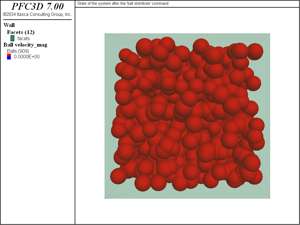
Figure 1: State of the system after the ball distribute command. Note the large overlaps.
The ball density and local damping coefficient are set with the ball attribute command. As presented in the “Attributes and Properties” tutorial, the density and local damping coefficient are attributes (not properties). The system is subsequently solved to an equilibrium criterion to achieve a dense packing.
ball attribute density 1000.0 damp 0.7
model cycle 2000 calm 10
model solve ratio-average 1e-3
model calm
Note that ball density is a required attribute, because a nonzero value is essential for PFC to properly resolve the equations of motion and compute a timestep. The local damping coefficient is set in this simulation to efficiently remove kinetic energy from the system, as we are interested in the final configuration. The model cycle command is given with the calm keyword to periodically null all ball translational/rotational velocities, effectively removing kinetic energy from the system. This allows the balls to be rearranged without significant overlap and without escaping the box, achieving a dense packing relatively rapidly. The model solve command is issued with a target average force ratio limit.
For further analysis, a measurement sphere is created and history monitoring is set up to record the evolution of the diagonal stresses within the assembly.
measure create id 1 radius 5.0
measure history name '1' stress-xx id 1
measure history name '2' stress-yy id 1
measure history name '3' stress-zz id 1
Figure 2 shows the system at this stage. Balls, walls, and the measurement sphere are plotted (the latter two being translated for convenience). The measurement sphere is colored by the calculated value of the porosity.
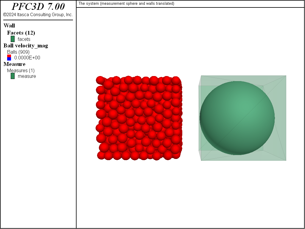
Figure 2: Initial state of the system before removing the walls. In this view, the walls and the measurement sphere are translated for convenience.
Now that a dense assembly of balls has been equilibrated, the next stage consists of installing parallel bonds in the system. This is done in two steps: (1) the contact method bond command is issued to bond contacts using a gap consistent with the settings of the CMAT slots above; and (2) the contact property command is issued to set the bond elasticity and strength properties.
contact method bond gap 0.1
contact property pb_kn 1e6 pb_ks 1e6 pb_ten 1e6 pb_coh 1e6 pb_fa 30.0
The initial state is now complete. The displacements are reset and the model state is saved.
ball attribute displacement multiply 0.0
model save 'initial'
Removing Confinement
At this stage, a parallel-bonded material has been created. We now alter the model by deleting the walls and solve the system to a target equilibrium criterion. Note that both linear springs and parallel bonds coexist at the ball-ball contacts.
wall delete
model cycle 1
model solve ratio-average 1e-3
model save 'final1'
Figure 3 shows the ball displacement vectors and force chains in the system. In the linear formulation, normal forces arise by default due to absolute overlap between model components. As a result, the linear springs were under compression in the presence of the walls. Contacts with parallel bonds, on the other hand, follow an incremental formulation for the normal force. Thus the parallel bonds act against imposed forces in an effort to return to their insertion configurations. When linear and parallel bonds are simultaneously present and the walls are removed, some of the load is transferred to stretching the parallel bonds.
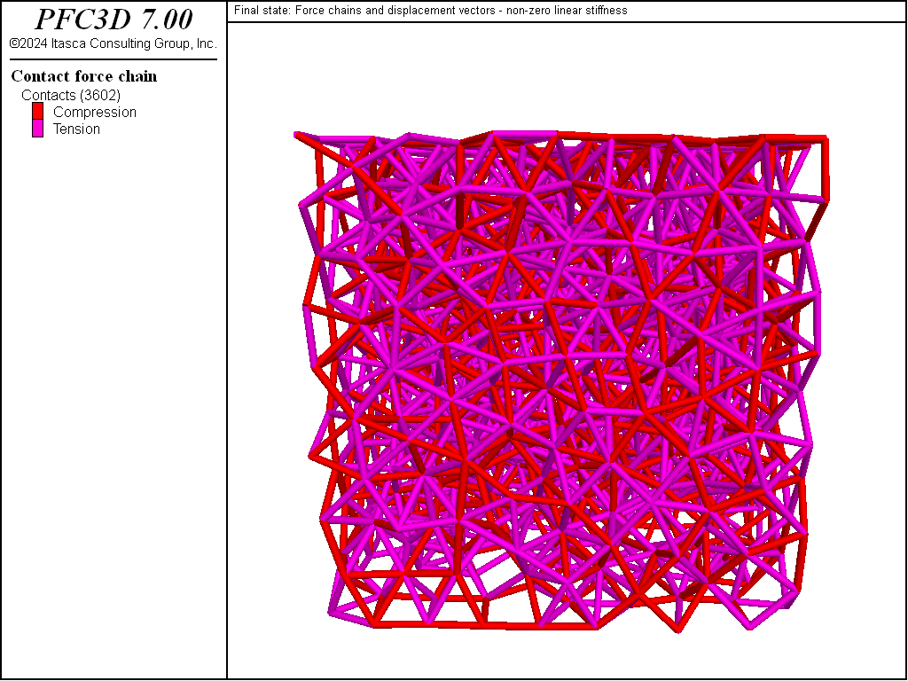
Figure 3: Final state after removing the walls and solving with linear stiffness. Force chains and ball displacements are shown.
Figure 4 shows the forces in the linear springs and in the contacts, while Figure 5 shows the evolution of the stresses within the assembly.
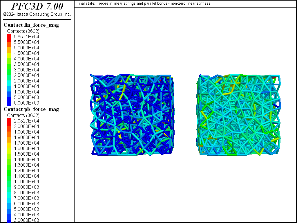
Figure 4: Final state after removing the walls and solving with linear stiffness. Forces in the linear spring (left) and in the parallel bonds (right, translated for convenience).
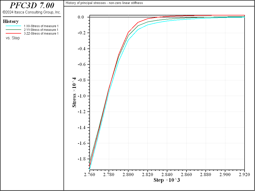
Figure 5: Histories of the principal stresses within the assembly computed with the measurement sphere, with nonzero linear stiffness.
The previous simulations involved both linear and parallel bond stiffnesses. Next we repeat the simulation but set the linear stiffnesses to 0.0. Thus there should be no forces present due to balls overlapping one another, and the model should be in equilibrium. Note, however, that there is a slight perturbation as forces previously accumulated to the balls act during the first cycle (Figures 6 to 8).
model restore 'initial'
wall delete
contact property kn 0.0
model cycle 1
model solve ratio-average 1e-3
model save 'final2'
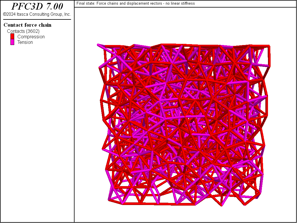
Figure 6: Final state after removing the walls and solving without linear stiffness. Force chains and ball displacements are shown.
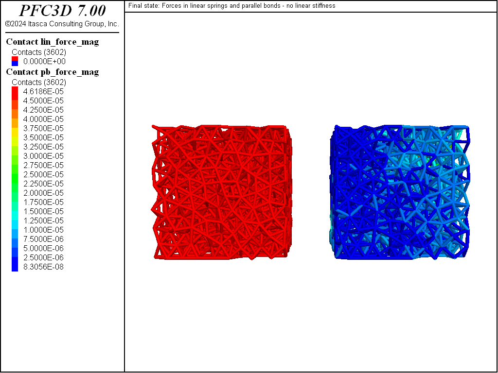
Figure 7: Final state after removing the walls and solving without linear stiffness. Forces in the linear spring (left) and in the parallel bonds (right).
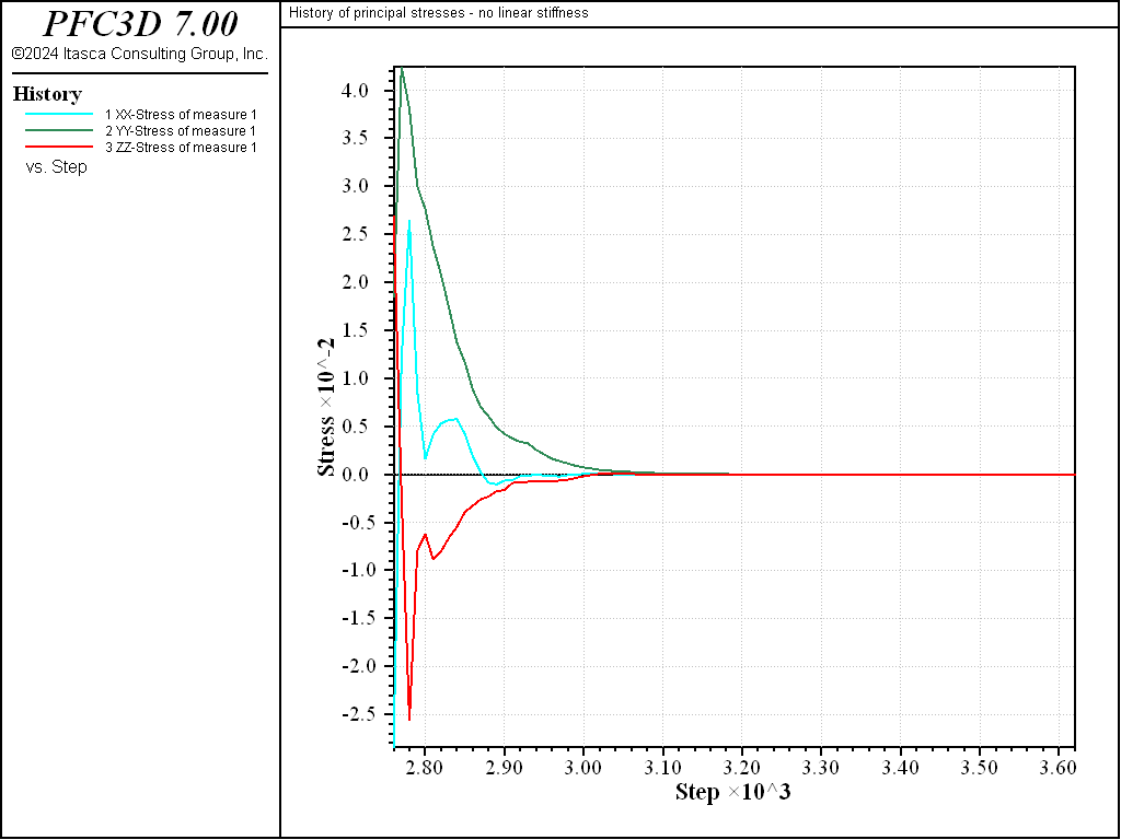
Figure 8: Histories of the principal stresses within the assembly computed with the measurement sphere, no linear stiffness.
To remove this perturbation, one must reset the contact forces (and possibly contact moments as well) that have been accumulated to the bodies during the previous force-displacement calculation cycle. For consistency, the lines below also reset the lin_force property of the linear parallel bond contact model (although this step is not mandatory).
model restore 'initial'
wall delete
contact property kn 0.0 lin_force 0.0 0.0 0.0
ball attribute force-contact multiply 0.0 moment-contact multiply 0.0
model cycle 1
model solve ratio-average 1e-3
model save 'final3'
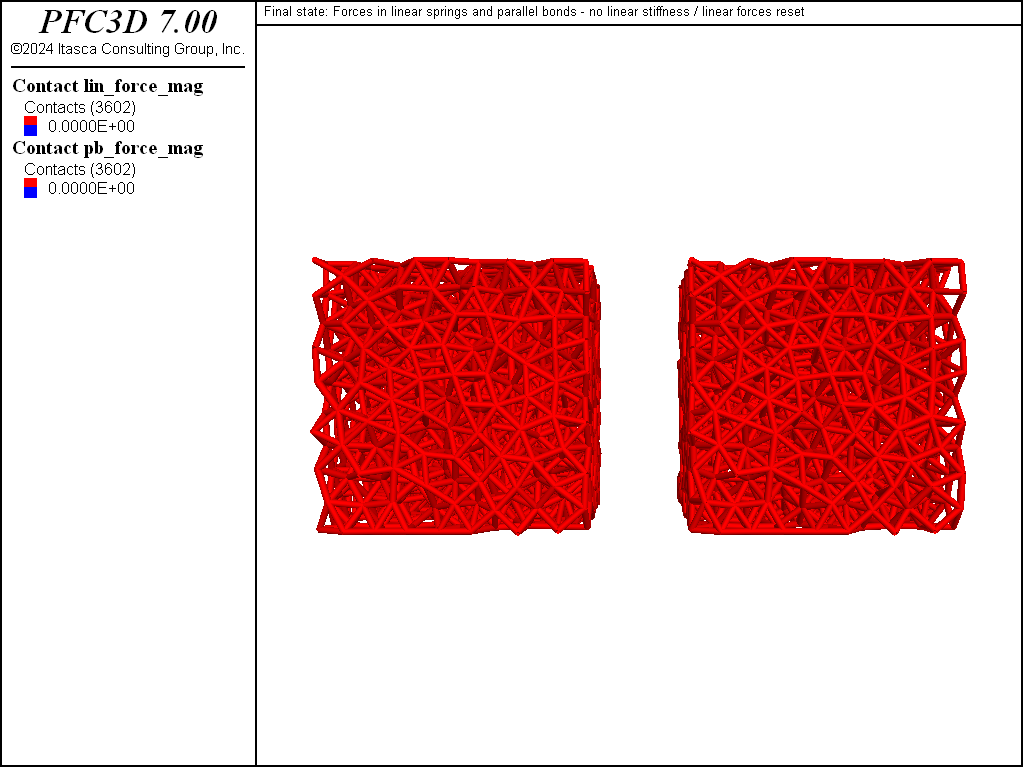
Figure 9: Final state after removing the walls and solving without linear stiffness and after a reset of the accumulated contact forces. Forces in the linear spring (left) and in the parallel bonds (right) are null.
Discussion
This example describes the steps to build a simple parallel-bonded material and the influence of the linear spring stiffness on the unconfined stage, and the final state has been illustrated. This is a rudimentary example to demonstrate the mechanics of using PFC for this bonded-particle modeling, highlighting some of the important features. Many additional steps are required to create a meaningful specimen to represent real materials (e.g., controlling the fabric of the initial state, calibrating material attributes and contact properties, etc.). Support for these additional steps is provided by the material-modeling support package.
References
| [Potyondy2015a] | Potyondy, D. O. “The Bonded-Particle Model as a Tool for Rock Mechanics Research and Application: Current Trends and Future Directions,” Geosystem Engineering, 18(1), 1–28 (2015), DOI:10.1080/12269328.2014.998346. |
Data Files
cmlinearpbond_simple.dat (3D)
; fname: cmlinearpbond_simpledat (3D)
;
;  Exercise the Linear Parallel Bond contact model
;=========================================================================
model new
model large-strain on
model title 'Generating a bonded assembly (Linear Parallel-Bond contact model)'

; Set the domain extent.
; excerpt-oiyv-start
model domain extent -10 10
; excerpt-oiyv-end

; Modify the default slots of the Contact Model Assignment Table (CMAT).
; Here we choose the linear contact model (with kn=1e6) for all contact
; types but ball-ball contacts, to which we assign the linearpbond model.
; Note that only the linear part of the linearpbond model is activated,
; therefore the model will exactly behave as the linear model.
; Also, the CMAT proximity distance is set to a non-zero value of 0.1 to
; ensure contacts are created when ball surfaces are within this distance.
; This setting should be consistent with the bond installation gap used below.
; excerpt-xwsu-start
contact cmat proximity 0.1
contact cmat default model linear property kn 1e6
contact cmat default type ball-ball model linearpbond property kn 1e6
; excerpt-xwsu-end

; Generate a box
; excerpt-gavv-start
wall generate box -5 5 one-wall
; excerpt-gavv-end

; Distribute balls in the box.
; The seed of the pseudo-random number generator is fixed, ensuring that the
; same initial configuration will be produced any time this file is executed.
;
; excerpt-fvvo-start
model random 10001
ball distribute porosity 0.36 radius 0.5 0.6 box -5 5
; excerpt-fvvo-end
model save 'balls'

; Set ball attributes.
; excerpt-unoa-start
ball attribute density 1000.0 damp 0.7
; excerpt-unoa-end

; Calm the system.
; Since the "ball distribute" command has been used above, the balls have
; been created without regard to the overlaps.
; excerpt-tdiw-start
model cycle 2000 calm 10
; excerpt-tdiw-end

; Solve the system to a target limit (here the average force ratio).
; excerpt-vluc-start
model solve ratio-average 1e-3
model calm
; excerpt-vluc-end

; Install a measurement sphere to monitor stresses within
; the assembly. Also reset ball displacements.
; excerpt-gpnu-start
measure create id 1 radius 5.0
measure history name '1' stress-xx id 1
measure history name '2' stress-yy id 1
measure history name '3' stress-zz id 1
; excerpt-gpnu-end

; Install parallel bonds - only contacts with linearpbond model are affected.
; A positive installation gap is positive, meaning that contacts with a gap
; less or equal to the specified value will be bonded. This setting should be
; consistent with the proximity distance priorly set in the CMAT.
; excerpt-exdr-start
contact method bond gap 0.1
contact property pb_kn 1e6 pb_ks 1e6 pb_ten 1e6 pb_coh 1e6 pb_fa 30.0
; excerpt-exdr-end

; Reset ball displacement and save the initial state.
; excerpt-kien-start
ball attribute displacement multiply 0.0
model save 'initial'
; excerpt-kien-end

; Delete the walls and solve to a target average ratio.
; excerpt-lqsl-start
wall delete
model cycle 1
model solve ratio-average 1e-3
model save 'final1'
; excerpt-lqsl-end

; Repeat the simulation but set the linear stiffness to 0.0.
; Note that the contact forces calculated at the previous timestep are
; already accumulated to the contacting balls - thus the slight perturbation
; from equilibrium.
; excerpt-vkrg-start
model restore 'initial'
wall delete
contact property kn 0.0
model cycle 1
model solve ratio-average 1e-3
model save 'final2'
; excerpt-vkrg-end

; Repeat the simulation but set the linear stiffness to 0.0
; and force a reset of the linear contact forces. All balls are fixed
; and the system is cycled for 1 step, to reset the linear forces.
; excerpt-stqj-start
model restore 'initial'
wall delete
contact property kn 0.0 lin_force 0.0 0.0 0.0
ball attribute force-contact multiply 0.0 moment-contact multiply 0.0
model cycle 1
model solve ratio-average 1e-3
model save 'final3'
; excerpt-stqj-end

program return
;========================================================================
; eof: cmlinearpbond_simple.dat (3D)
Endnotes
| [1] | To view this project in PFC, use the program menu.
⮡ PFC |
| Was this helpful? ... | FLAC3D © 2019, Itasca | Updated: Feb 25, 2024 |
