Linear Parallel Bond Model
The linear parallel bond model with inactive dashpots and a reference gap of zero corresponds with the parallel-bond model of [Potyondy2004]. It is a linear-based model that can be installed at both ball-ball and ball-facet contacts and is referred to in commands and FISH by the name linearpbond.
Introduction
A parallel bond provides the mechanical behavior of a finite-sized piece of cement-like material deposited between the two contacting pieces (similar to the epoxy cementing the glass beads shown in Figure 2). The parallel-bond component acts in parallel with the linear component and establishes an elastic interaction between the pieces. The existence of a parallel bond does not preclude the possibility of slip. Parallel bonds can transmit both force and moment between the pieces.
A parallel bond can be envisioned as a set of elastic springs with constant normal and shear stiffnesses, uniformly distributed over a {rectangular in 2D; circular in 3D} cross-section lying on the contact plane and centered at the contact point. These springs act in parallel with the springs of the linear component. Relative motion at the contact, occurring after the parallel bond has been created, causes a force and moment to develop within the bond material. This force and moment act on the two contacting pieces and can be related to maximum normal and shear stresses acting within the bond material at the bond periphery. If either of these maximum stresses exceeds its corresponding bond strength, the parallel bond breaks, and the bond material is removed from the model along with its accompanying force, moment, and stiffnesses.
Behavior Summary
The linear parallel bond model provides the behavior of two interfaces: an infinitesimal, linear elastic (no-tension), and frictional interface that carries a force and a finite-size, linear elastic, and bonded interface that carries a force and moment (see Figure 1). The first interface is equivalent to the linear model: it does not resist relative rotation, and slip is accommodated by imposing a Coulomb limit on the shear force. The second interface is called a parallel bond, because when bonded, it acts in parallel with the first interface. When the second interface is bonded, it resists relative rotation, and its behavior is linear elastic until the strength limit is exceeded and the bond breaks, making it unbonded. When the second interface is unbonded, it carries no load. The unbonded linear parallel bond model is equivalent to the linear model.
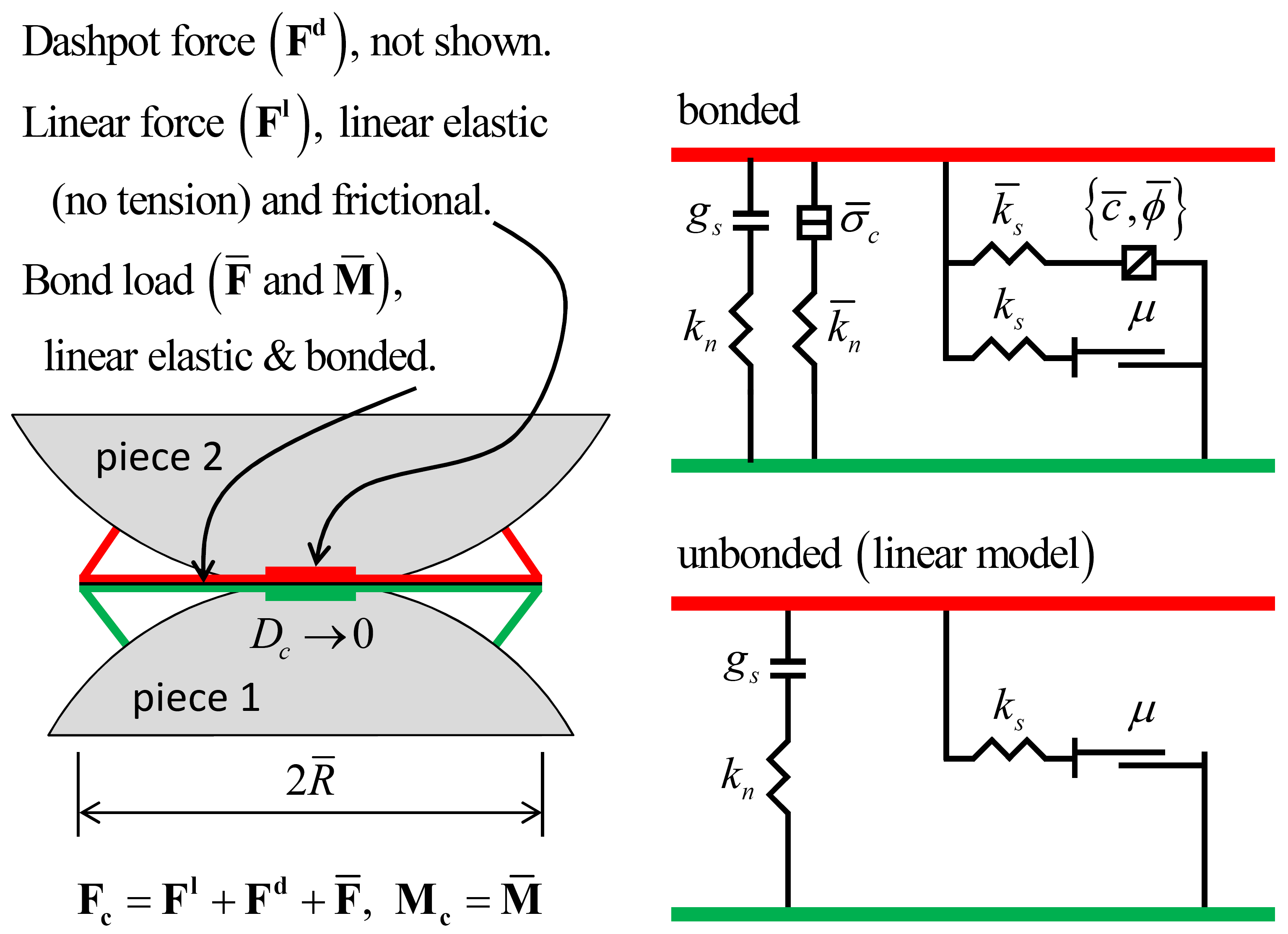
Figure 1: Behavior and rheological components of the linear parallel bond model with inactive dashpots.
Activity-Deletion Criteria
A contact with the linear parallel bond model is active if it is bonded or if the surface gap is less than or equal to zero. The force-displacement law is skipped for inactive contacts. The surface gap is shown in this figure of the linear formulation. When the reference gap is zero, the notional surfaces of the first interface coincide with the piece surfaces. The notional surfaces of the second interface are shown in Figure 2.
Force-Displacement Law
The force-displacement law for the linear parallel bond model updates the contact force and moment:
where \(\mathbf{F^{l}}\) is the linear force, \(\mathbf{F^{d}}\) is the dashpot force, \(\overline{\mathbf{F}}\) is the parallel-bond force, and \(\overline{\mathbf{M}}\) is the parallel-bond moment. The linear and dashpot forces are updated as in the linear model, while the force and moment in the parallel bond are updated as described below.
The parallel-bond force is resolved into a normal and shear force, and the parallel-bond moment is resolved into a twisting and bending moment:
where \(\overline{F}_{n} > 0\) is tension. The parallel-bond shear force and bending moment lie on the contact plane and are expressed in the contact plane coordinate system:
When a parallel bond is created via the bond method, an interface between two notional surfaces is established, and the parallel-bond force and moment are zeroed. The parallel bond provides an elastic interaction between these two notional surfaces, and this interaction is removed when the bond breaks. Each notional surface is connected rigidly to the piece of a body as shown in Figure 2. The parallel-bond surface gap is defined as the cumulative relative normal displacement of the piece surfaces:
where \(\Delta \delta _{n}\) is the relative normal-displacement increment of this equation of the “Contact Resolution” section.
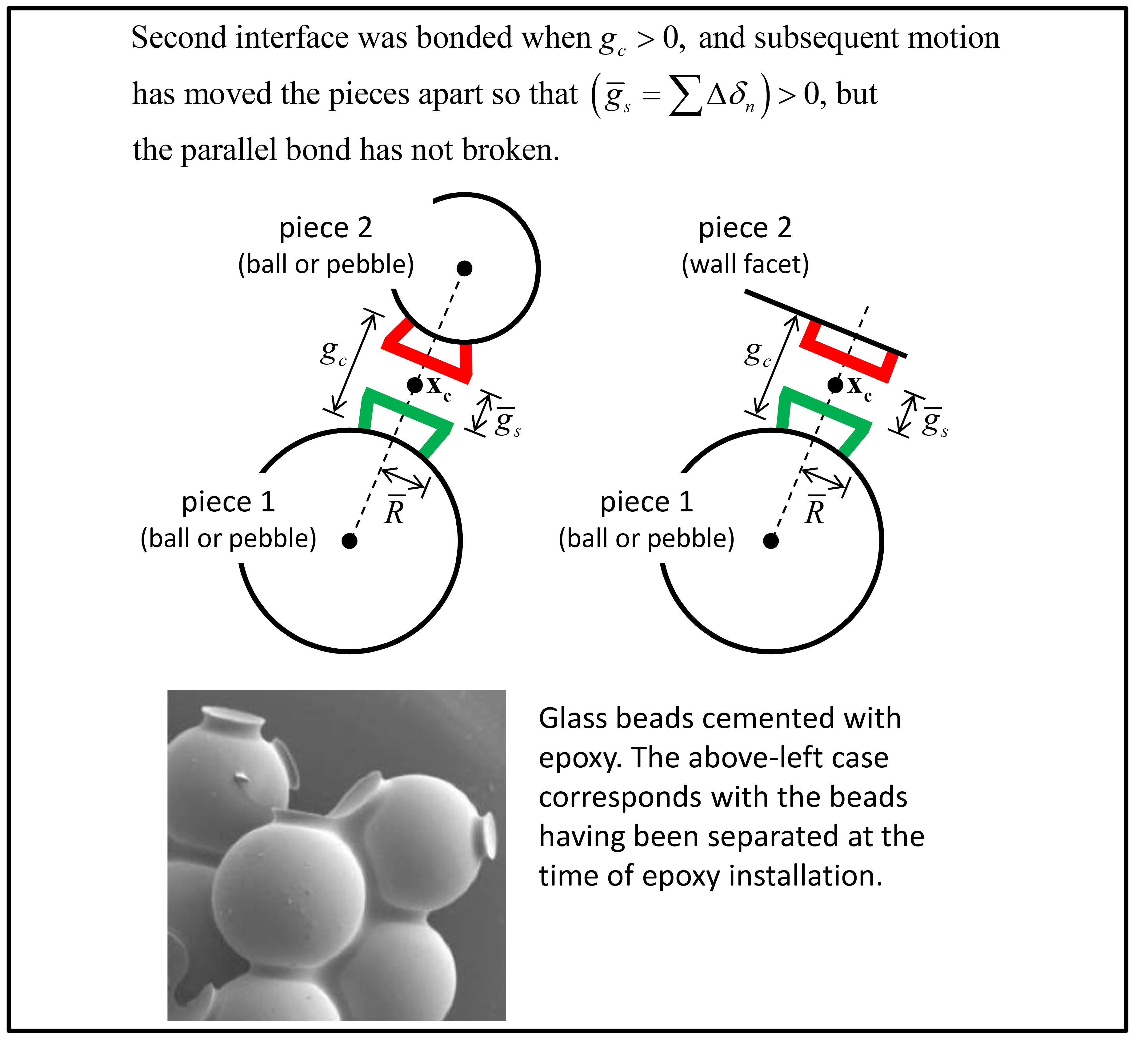
Figure 2: Finite-size notional surfaces (green and red) and parallel-bond surface gap at parallel-bonded ball-ball (left) and ball-facet (right) contacts. (Photograph of glass beads from [Holt2005].)
The force-displacement law for the parallel-bond force and moment consists of the following steps (see Figure 3).
Update the bond cross-sectional properties:
(5)\[\begin{split}\begin{array}{c} \overline{R} = \overline{\lambda} \left\{ \begin{array}{rl} \min\left( R^{(1)}, R^{(2)} \right), & \mbox{ball-ball} \\ R^{(1)}, & \mbox{ball-facet} \end{array} \right. ,\quad \overline{A} = \left\{ \begin{array}{rl} 2 \bar{R} t, & \mbox{2D $(t = 1)$} \\ \pi \bar{R}^2, & \mbox{3D} \end{array} \right. \\[3mm] \overline{I} = \left\{ \begin{array}{rl} \tfrac{2}{3} t \bar{R}^3, & \mbox{2D $(t = 1)$} \\ \tfrac{1}{4} \pi \bar{R}^4, & \mbox{3D} \end{array} \right. ,\quad \overline{J} = \left\{ \begin{array}{rl} 0, & \mbox{2D} \\ \tfrac{1}{2} \pi \bar{R}^4, & \mbox{3D} \end{array} \right. \end{array}\end{split}\]where \(\overline{A}\) is the cross-sectional area, \(\overline{I}\) is the moment of inertia of the parallel bond cross section (about the line passing through \(\mathbf{x_{c}}\) and in the direction of \(\overline{\mathbf{M}}_\mathbf{b}\)), and \(\overline{J}\) is the polar moment of inertia of the parallel bond cross section (about the line passing through \(\mathbf{x_{c}}\) and in the direction of \(\hat{\mathbf{n}}_\mathbf{c}\)). The bond cross section is {rectangular in 2D; circular in 3D}.
Update \(\overline{F}_n\):
(6)\[\overline{F}_{n} :=\overline{F}_{n} +\overline{k}_{n} {\kern 1pt} \overline{A}\, \Delta \delta _{n}\]where \(\Delta \delta _{n}\) is the relative normal-displacement increment of this equation of the “Contact Resolution” section.
Update \(\overline{\mathbf{F}}_\mathbf{s}\):
(7)\[\overline{\mathbf{F}}_\mathbf{s} :=\overline{\mathbf{F}}_\mathbf{s} -\overline{k}_{s} {\kern 1pt} \overline{A}{\kern 1pt} \Delta \pmb{δ} _\mathbf{s}\]where \(\Delta \pmb{δ}_\mathbf{s}\) is the relative shear-displacement increment of this equation of the “Contact Resolution” section.
Update \(\overline{M}_{t}\):
(8)\[\begin{split} \overline{M}_t := \left\{ \begin{array}{rl} 0, & \mbox{2D} \\ \overline{M}_t - \overline{k}_s \overline{J} \Delta \theta_t, & \mbox{3D} \end{array} \right.\end{split}\]where \(\Delta \theta _{t}\) is the relative twist-rotation increment of this equation of the “Contact Resolution” section. The torsional stiffness \((k_{t})\) of a twisted elastic circular shaft of length \(L\) loaded at its ends by equal and opposite twisting moments is given by [Crandall1978] (Eq. 6.10):
(9)\[M_{t} =k_{t} \theta _{t} ,\quad k_{t} =\frac{GJ}{L}\]where \(G\) is the shear modulus and \(J\) is the polar moment of inertia of the cross-sectional area about the axis of the shaft. The moment-twist relation of Equation (8) is obtained by setting \(k_{t} =\overline{k}_{s} {\kern 1pt} \overline{J}\).
Update \(\overline{\mathbf{M}}_\mathbf{b}\):
(10)\[\overline{\mathbf{M}}_\mathbf{b} := \overline{\mathbf{M}}_\mathbf{b} - \overline{k}_{n} {\kern 1pt} \overline{I}{\kern 1pt} \Delta \pmb{θ}_\mathbf{b}\]where \(\Delta \pmb{θ}_\mathbf{b}\) is the relative bend-rotation increment of this equation of the “Contact Resolution” section. The bending stiffness \(\left(k_{b} \right)\) of an elastic symmetrical beam of length \(L\) loaded at its ends by equal and opposite bending moments is given by [Crandall1978] (Eq. 7.14):
(11)\[M_{b} =k_{b} \theta _{b} ,\quad k_{b} =\frac{EI}{L}\]where \(E\) is the Young’s modulus and \(I\) is the moment of inertia of the cross-sectional area about the neutral axis of the beam. The moment-twist relation of Equation (11) is obtained by setting \(k_{b} =\overline{k}_{n} {\kern 1pt} \overline{I}\).
Update the maximum normal (\(\overline{\sigma}\), \(\overline{\sigma} > 0\) is tension) and shear stresses at the parallel-bond periphery:
(12)\[\begin{split}\begin{array}{l} \overline{\sigma} = \displaystyle\frac{\overline{F}_n}{\overline{A}} + \overline{\beta} \frac{\left\| \overline{\mathbf{M}}_\mathbf{b} \right\| \overline{R}}{\overline{I}} ,\quad \overline{\tau} = \frac{\left\| \overline{\mathbf{F}}_\mathbf{s} \right\|}{\overline{A}} + \left\{ \begin{array}{rl} 0, & \mbox{2D} \\ \overline{\beta} \frac{\left| \overline{M}_t \right| \overline{R}}{\overline{J}}, & \mbox{3D} \end{array} \right. \\[1mm] \mbox{with }\quad \overline{\beta} \in [0, 1]. \end{array}\end{split}\]The moment-contribution factor \(\left( \overline{\beta } \right)\) is discussed in [Potyondy2011].
Enforce the strength limits (see Figure 4). If the tensile-strength limit is exceeded \(\left(\overline{\sigma }>\overline{\sigma }_{c} \right)\), then break the bond in tension:
(13)\[\overline{B}=1,\quad \left\{\overline{F}_{n} ,\overline{F}_{ss} ,\overline{F}_{st} ,\overline{M}_{t} ,\overline{M}_{bs} ,\overline{M}_{bt} \right\}=0.\]If the bond has not broken in tension, then enforce the shear-strength limit. The shear strength \(\overline{\tau}_{c} = \overline{c} - \sigma \tan \overline{\phi}\), where \(\sigma = \overline{F}_{n} / \overline{A}\) is the average normal stress acting on the parallel bond cross section. If the shear-strength limit is exceeded \((\overline{\tau} > \overline{\tau}_{c})\), then break the bond in shear:
(14)\[\overline{B}=2,\quad \left\{\overline{F}_{n} ,\overline{F}_{ss} ,\overline{F}_{st} ,\overline{M}_{t} ,\overline{M}_{bs} ,\overline{M}_{bt} \right\}=0.\]If the bond has broken, then the bond_break callback event is triggered.
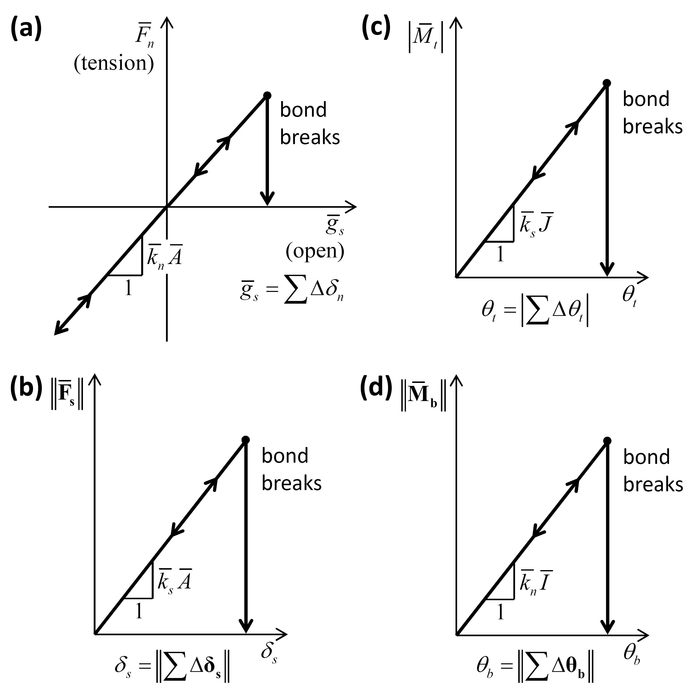
Figure 3: Force-displacement law for the parallel bond force and moment: (a) normal force versus parallel-bond surface gap; (b) shear force versus relative shear displacement; (c) twisting moment versus relative twist rotation; and (d) bending moment versus relative bend rotation.
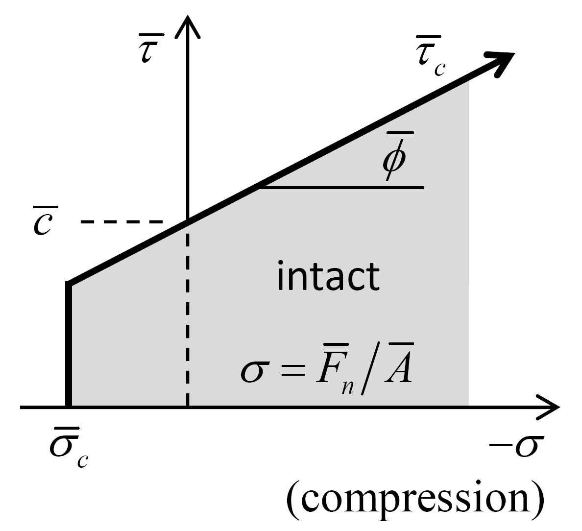
Figure 4: Failure envelope for the parallel bond.
Energy Partitions
The linear parallel bond model provides four energy partitions:
- strain energy, \(E_{k}\), stored in the linear springs;
- slip energy, \(E_{\mu }\), defined as the total energy dissipated by frictional slip;
- dashpot energy, \(E_{\beta }\), defined as the total energy dissipated by the dashpots; and
- bond strain energy, \(\overline{E}_k\), stored in the parallel-bond springs.
| Keyword | Symbol | Description | Range | Accumulated |
|---|---|---|---|---|
| Linear Group: | ||||
energy‑strain |
\(E_{k}\) | strain energy | \([0.0,+\infty)\) | NO |
energy‑slip |
\(E_{\mu}\) | total energy dissipated by slip | \((-\infty,0.0]\) | YES |
| Dashpot Group: | ||||
energy‑dashpot |
\(E_{\beta}\) | total energy dissipated by dashpots | \((-\infty,0.0]\) | YES |
| Parallel-Bond Group: | ||||
energy‑epbstrain |
\(\overline{E}_k\) | bond strain energy | \([0.0,+\infty)\) | NO |
The strain energy, slip energy, and dashpot energy are updated as for the linear model (see this section). The slip energy remains equal to zero until the bond breaks. The bond strain energy is updated via:
Properties
The properties defined by the linear parallel bond model are listed in the table below for a concise reference; see the “Contact Properties” section for a description of the information in the table columns. The mapping from the surface inheritable properties to the contact model properties is also discussed below.
| Keyword | Symbol | Description | Type | Range | Default | Modifiable | Inheritable |
|---|---|---|---|---|---|---|---|
| linearpbond | Model name | ||||||
| Linear Group: | |||||||
| kn | \(k_n\) | Normal stiffness [force/length] | FLT | \([0.0,+\infty)\) | 0.0 | YES | YES |
| ks | \(k_s\) | Shear stiffness [force/length] | FLT | \([0.0,+\infty)\) | 0.0 | YES | YES |
| fric | \(\mu\) | Friction coefficient [-] | FLT | \([0.0,+\infty)\) | 0.0 | YES | YES |
| rgap | \(g_r\) | Reference gap [length] | FLT | \(\mathbb{R}\) | 0.0 | YES | NO |
| lin_mode | \(M_l\) | Normal-force update mode [-] | INT | \(\{0,1\}\) | 0 | YES | NO |
| \(\;\;\;\;\;\;\begin{cases} \mbox{0: update is absolute} \\ \mbox{1: update is incremental} \end{cases}\) | |||||||
| emod | \(E^*\) | Effective modulus [force/area] | FLT | \([0.0,+\infty)\) | 0.0 | NO | N/A |
| kratio | \(\kappa^*\) | Normal-to-shear stiffness ratio [-] | FLT | \([0.0,+\infty)^*\) | 0.0\(^*\) | NO | N/A |
| \(\kappa^* \equiv \frac{k_n}{k_s}\) | |||||||
| lin_slip | \(s\) | Slip state [-] | BOOL | {false,true} | false | NO | N/A |
| \(\;\;\;\;\;\;\begin{cases} \mbox{true: slipping} \\ \mbox{false: not slipping} \end{cases}\) | |||||||
| lin_force | \(\mathbf{F^l}\) | Linear force (contact plane coord. system) | VEC | \(\mathbb{R}^3\) | \(\mathbf{0}\) | YES | NO |
| \(\left( -F_n^l,F_{ss}^l,F_{st}^l \right) \quad \left(\mbox{2D model: } F_{ss}^l \equiv 0 \right)\) | |||||||
| user_area | \(A\) | Constant area [length*length] | FLT | \((0.0,+\infty)\) | 0.0 | YES | NO |
| Dashpot Group: | |||||||
| dp_nratio | \(\beta_n\) | Normal critical damping ratio [-] | FLT | \([0.0,1.0]\) | 0.0 | YES | NO |
| dp_sratio | \(\beta_s\) | Shear critical damping ratio [-] | FLT | \([0.0,1.0]\) | 0.0 | YES | NO |
| dp_mode | \(M_d\) | Dashpot mode [-] | INT | {0,1,2,3} | 0 | YES | NO |
| \(\;\;\;\;\;\;\begin{cases} \mbox{0: full normal & full shear} \\ \mbox{1: no-tension normal & full shear} \\ \mbox{2: full normal & slip-cut shear} \\ \mbox{3: no-tension normal & slip-cut shear} \end{cases}\) | |||||||
| dp_force | \(\mathbf{F^d}\) | Dashpot force (contact plane coord. system) | VEC | \(\mathbb{R}^3\) | \(\mathbf{0}\) | NO | NO |
| \(\left( -F_n^d,F_{ss}^d,F_{st}^d \right) \quad \left(\mbox{2D model: } F_{ss}^d \equiv 0 \right)\) | |||||||
| Parallel-Bond Group: | |||||||
| pb_rmul | \(\overline{\lambda}\) | Radius multiplier [-] | FLT | \((0.0,+\infty)\) | 1.0 | YES | NO |
| pb_kn | \(\overline{k}_n\) | Normal stiffness [stress/disp.] | FLT | \([0.0,+\infty)\) | 0.0 | YES | NO |
| pb_ks | \(\overline{k}_s\) | Shear stiffness [stress/disp.] | FLT | \([0.0,+\infty)\) | 0.0 | YES | NO |
| pb_mcf | \(\overline{\beta}\) | Moment-contribution factor [-] | FLT | \([0.0,1]\) | 1.0 | YES | NO |
| pb_ten | \(\overline{\sigma}_c\) | Tensile strength [stress] | FLT | \([0.0,+\infty)\) | 0.0 | YES | NO |
| pb_coh | \(\overline{c}\) | Cohesion [stress] | FLT | \([0.0,+\infty)\) | 0.0 | YES | NO |
| pb_fa | \(\overline{\phi}\) | Friction angle [degrees] | FLT | \([0.0,90.0)\) | 0.0 | YES | NO |
| pb_state | \(\overline{B}\) | Bond state | INT | {0,1,2,3} | 0 | NO | NO |
| \(\;\;\;\;\;\;\begin{cases} \mbox{0: unbonded} \\ \mbox{1: unbonded & broke in tension} \\ \mbox{2: unbonded & broke in shear} \\ \mbox{3: bonded} \end{cases}\) | |||||||
| pb_radius | \(\overline{R}\) | Bond radius [length] | FLT | \((0.0,+\infty)\) | N/A | NO (set via \(\overline{\lambda}\)) | NO |
| pb_emod | \(\overline{E}^{*}\) | Bond effective modulus [stress] | FLT | \([0.0,+\infty)\) | 0.0 | NO | N/A |
| pb_kratio | \(\overline{\kappa }^{*}\) | Bond normal-to-shear stiffness ratio | FLT | \([0.0,+\infty)^{*}\) | 0.0 | NO | N/A |
| \(\overline{\kappa}^* \equiv \frac{\overline{k}_n}{\overline{k}_s}\) | |||||||
| pb_shear | \(\overline{\tau }_{c}\) | Bond shear strength [stress] | FLT | \([0.0,+\infty)\) | 0.0 | NO (set via \(\overline{c}\) and \(\overline{\sigma}_c\)) | N/A |
| pb_sigma | \(\overline{\sigma }\) | Normal stress at bond periphery [stress] | FLT | \([0.0,+\infty)\) | 0.0 | NO | N/A |
| pb_tau | \(\overline{\tau }\) | Shear stress at bond periphery [stress] | FLT | \([0.0,+\infty)\) | 0.0 | NO | N/A |
| pb_force | \(\overline{\mathbf{F}}\) | Parallel-bond force (contact plane coord. system) | VEC | \(\mathbb{R}^3\) | \(\mathbf{0}\) | YES | NO |
| \(\left( -\overline{F}_n,\overline{F}_{ss},\overline{F}_{st} \right) \quad \left(\mbox{2D model: } \overline{F}_{ss} \equiv 0 \right)\) | |||||||
| pb_moment | \(\overline{\mathbf{M}}\) | Parallel-bond moment (contact plane coord. system) | VEC | \(\mathbb{R}^3\) | \(\mathbf{0}\) | YES | NO |
| \(\left( \overline{M}_t,\overline{M}_{bs},\overline{M}_{bt} \right) \quad \left(\mbox{2D model: } \overline{M}_{t} \equiv \overline{M}_{bt} \equiv 0 \right)\) | |||||||
| \(^*\) By convention, \(\kappa^*\) and \(\overline{\kappa }^{*}\) equal zero if either corresponding normal or shear stiffness is zero. | |||||||
Note
Modifying the contact model force will not alter forces accumulated to the bodies. Therefore, any change to \(\mathbf{F^l}\), \(\overline{\mathbf{F}}\), or \(\overline{\mathbf{M}}\) may only be effective during the next force-displacement calculation. When \(M_l = 0\), the normal component of the linear force is automatically overridden during the next force-displacement calculation.
Surface Property Inheritance
The linear stiffnesses, \(k_n\) and \(k_s\), and the friction coefficient, \(\mu\), may be inherited from the contacting pieces. See this section from the linear formulation for details on property inheritance.
Methods
| Method | Arguments | Symbol | Type | Range | Default | Description | |
|---|---|---|---|---|---|---|---|
| Linear Group: | |||||||
| area | Set user_area to the area | |||||||
| deformability | Set deformability | |||||||
| emod | \(E^*\) | FLT | \([0.0,+\infty)\) | N/A | Effective modulus | ||
| kratio | \(\kappa^*\) | FLT | \([0.0,+\infty)^*\) | N/A | Normal-to-shear stiffness ratio | ||
| Parallel-Bond Group: | |||||||
| pb_deformability | Set bond deformability | ||||||
| emod | \(\overline{E}^*\) | FLT | \([0.0,+\infty)\) | N/A | Bond effective modulus | ||
| kratio | \(\overline{\kappa}^*\) | FLT | \([0.0,+\infty)^*\) | N/A | Bond normal-to-shear stiffness ratio, \(\overline{\kappa}^* \equiv \frac{\overline{k}_n}{\overline{k}_s}\) | ||
| bond | Bond the contact if \(g_c \in G\) | ||||||
| gap | \(G\) | VEC2 | \(\mathbb{R}^2\) | \((-\infty,0]\) | Gap interval | ||
| unbond | Unbond the contact if \(g_c \in G\) | ||||||
| gap | \(G\) | VEC2 | \(\mathbb{R}^2\) | \((-\infty,0]\) | Gap interval | ||
| \(^*\) By convention, setting \(\kappa^*\) and \(\overline{\kappa }^{*}\) equal to zero sets the corresponding shear stiffness to zero but does not modify the corresponding normal stiffness. | |||||||
Area
Set the user_area property via the current contact area. This operation means that the contact area stays constant and is fixed independent of changes to the piece sizes/geometries. In order for the stiffnesses to be recomputed accounting for this area, one should subsequently call the deformabilty and/or pb_deformability methods.
Deformability
See this section from the linear formulation for details on this method.
pb_deformability
The deformability provided by the first interface can be specified with the deformability method. The additional deformability provided by the parallel bond can be specified with the pb_deformability method, which sets
The first term in this expression is obtained by equating the normal stiffness to the axial stiffness of the volume of material shown in this figure of the linear model formulation.
Bond
Create a parallel bond by bonding the second interface if the contact gap between the pieces is within the bonding-gap interval. If no gap is specified, then the second interface is bonded if the pieces overlap. A single value can be specified with the gap keyword corresponding to the maximum gap. One can ensure the existence of contacts between all pieces with a contact gap less than a specified bonding gap \((g_b)\) by specifying \(g_b\) with the proximity in the contact cmat default command of the Contact Model Assignment Table (CMAT). If the second interface becomes bonded, then the parallel bond force, moment and surface gap are zeroed.
Unbond
Remove a parallel bond by unbonding the second interface if the contact gap between the pieces is within the bonding-gap interval. If no gap is specified, then the second interface is unbonded if the pieces overlap. A single value can be specified with the gap keyword corresponding to the maximum gap. If the second interface becomes unbonded, then the bond state becomes unbonded \((\overline{B}=0)\). The parallel bond force and moment are unaffected and will be updated during the next cycle.
Callback Events
| Event | Array Slot | Value Type | Range | Description |
|---|---|---|---|---|
| contact_activated | Contact has become active | |||
| 1 | C_PNT | N/A | Contact pointer | |
| Linear Group: | ||||
| slip_change | Slip state has changed | |||
| 1 | C_PNT | N/A | Contact pointer | |
| 2 | INT | {0,1} | Slip change mode | |
| \(\;\;\;\;\;\;\begin{cases} \mbox{0: slip has initiated} \\ \mbox{1: slip has ended} \end{cases}\) | ||||
| Parallel-Bond Group | ||||
| bond_break | Bond has broken | |||
| 1 | C_PNT | N/A | Contact pointer | |
| 2 | INT | {1,2} | Failure mode | |
| \(\;\;\;\;\;\;\begin{cases} \mbox{1: failed in tension} \\ \mbox{2: failed in shear} \end{cases}\) | ||||
| 3 | FLT | \([0.0,+\infty)\) | Failure strength [force] (\(\overline{\sigma }_{c}\) or \(\overline{\tau }_{c}\), according to the failure mode) | |
| 4 | FLT | \([0.0,+\infty)\) | Bond strain energy \(\overline{E}_k\) at onset of failure | |
Usage and Verification Examples
The tutorial example “Generating a Bonded Assembly” demonstrates the use of the linear parallel bond model.
The verification problem “Tip-Loaded Cantilever Beam” uses the linear parallel bond contact model to model a cantilever beam and compares its mechanical response to load against analytical solutions.
The example “Rock Testing” compares the response of a parallel bonded material under typical laboratory testing conditions (unconfined compression and direct-tension tests) with that of flat-jointed material.
The tutorial example “Inclusions in a Matrix” also uses the linear parallel bond model. Its purpose is to illustrate how material regions with different mechanical properties may be created.
The tutorial examples “Creation of a Synthetic Rock Mass (SRM) Specimen” and “Slip on a Fault” illustrate how interfaces may be inserted in a parallel bonded material and modeled using the Smooth-Joint Model.
Model Summary
An alphabetical list of the linear parallel bond contact model methods is given here. An alphabetical list of the linear parallel bond contact model properties is given here.
References
| [Crandall1978] | (1, 2) Crandall, S.H., N.C. Dahl and T.J. Lardner. “An Introduction to the Mechanics of Solids, Second Edition,” New York: McGraw-Hill Book Company. |
| [Holt2005] | Holt, R.M., J. Kjølass, I. Larsen, L. Li, A. Gotusso Pillitteri and E.F. Sønstebø. “Comparison Between Controlled Laboratory Experiments and Discrete Particle Simulations of the Mechanical Behavior of Rock,” Int. J. Rock Mech. Min. Sci., 42, 985-995. |
| [Potyondy2011] | Potyondy, D.O. “Parallel-Bond Refinements to Match Macroproperties of Hard Rock,” in Continuum and Distinct Element Numerical Modeling in Geomechanics 2011 (Proceedings of Second International FLAC/DEM Symposium, Melbourne, Australia, 14–16 February 2011), pp. 459–465. D. Sainsbury, R. Hart, C. Detournay and M. Nelson, Eds. ISBN 978-0-9767577-2-6. Minneapolis: Itasca International. |
| Was this helpful? ... | FLAC3D © 2019, Itasca | Updated: Feb 25, 2024 |