One-way Fluid Coupling

For some problems, it is desirable to use some form of one-way coupling. In one-way coupling, the particles are influenced by the fluid, but the fluid is not influenced by the particles. The CFD module supports this type of modeling. The basic procedure is the following.

• Read a fluid mesh.
• Set the fluid density and viscosity.
• Set the fluid velocity.
• Solve or cycle.

Problem Description

Three particles with radii 1, 1.5 and 2 mm and density 2000 kg/m³ settle under gravity in a still fluid with density 1000 kg/m³ and viscosity of 1.5 Pa s.

Analytical Solution

The equation of motion for a spherical particle falling under gravity in a viscous fluid is

(1)\[{4 \over 3}\pi r^3 \rho_p {du_z \over {dt}} = {4 \over 3}\pi r^3\left(\rho_p-\rho_f\right)g - {1 \over 2}\pi r^2\rho_f C_d u_z^2\]

where \(g\) is the acceleration due to gravity, \(\rho_p\) and \(f\) are the particle and fluid densities, \(u_z\) is the vertical velocity of the settling particle, and \(C_d\) is the drag coefficient. The drag coefficient, \(C_d\), is a function of the particle Reynolds number.

As the falling ball reaches a steady velocity, \(du_z \over dt\) becomes zero. This allows us to write

(2)\[{1 \over 2}\pi r^2\rho_f C_d u_z^2 = {4 \over 3}\pi r^3 \left(\rho_p - \rho_f\right) g\]

It has been shown that for small Reynolds numbers, the drag coefficient is simply ([Batchelor1967])

(3)\[C_d = {24 \over Re_p}\]

where \(Re_p\) is the particle Reynolds number defined as

(4)\[Re_p = {{2r \rho_f u_z} \over {\mu_f}}\]

With this definition of \(C_d\), Equation (1) can be solved exactly to give Stokes’ law:

(5)\[u_z = {2 \over 9} {{r^2(\rho_p-\rho_f)g} \over {\mu_f}} \ \ \ \ \ {\rm for} \ Re_p \ll 1\]

Implementation

The file one_way_cfd.p3dat listed below drives this example.

model new
model large-strain on
model title 'One-way CFD coupling example'
model domain extent -1 2 -1 2 0 2 condition periodic
contact cmat default model linear
model mechanical timestep max 1e-5

wall generate name 'cell1' box 0 1 0 1 0 1
wall delete walls range set name 'cell1Bottom'
wall delete walls range set name 'cell1Top'
wall generate name 'cell2' box 0 1 0 1 1 2
wall delete walls range set name 'cell2Bottom'
wall delete walls range set name 'cell2Top'
wall property 'kn' 1e2 'ks' 1e2 'fric' 0.25

model gravity 0 0 -9.81

ball create radius 0.001  position-x 0.5 position-y 0.3  position-z 1.5
ball create radius 0.0015 position-x 0.5 position-y 0.5  position-z 1.5
ball create radius 0.002  position-x 0.5 position-y 0.7  position-z 1.5

ball attribute density 2000.0
ball property 'kn' 1e2 'ks' 1e2 'fric' 0.25

model configure cfd

cfd read nodes 'Node.dat'
cfd read elements 'Elem.dat'
cfd buoyancy on
element cfd attribute density 1000.0
element cfd attribute viscosity 1.5

element cfd attribute velocity-x 0.0
element cfd attribute velocity-y 0.0
element cfd attribute velocity-z 0.0

fish define set_fluid_velocity
  loop foreach local ele element.cfd.list
    element.cfd.vel.x(ele) = 0.0
    element.cfd.vel.y(ele) = 0.0
    element.cfd.vel.z(ele) = 0.0
  end_loop
end
[set_fluid_velocity]

ball history velocity-z id 1
ball history velocity-z id 2
ball history velocity-z id 3
model cycle 2500
ball list attribute velocity
program return

Once the CFD module has been loaded with the command model configure cfd, the fluid particle interaction forces will be calculated and applied to the particles.

Results

The three different particles reach three different terminal velocities. This is expected since the terminal velocity is controlled by a balance between drag forces which are proportional to particle radius squared and gravitational forces which are proportional to particle radius cubed.

The PFC particle terminal velocities are -1.50, -3.33 and -5.86 mm/s. Stokes’ law (5) predicts terminal velocities of -1.45, -3.27 and -5.81 mm/s. PFC predicts slightly higher terminal velocities than Stokes’ law because the drag coefficient formulation used in PFC includes momentum effects.

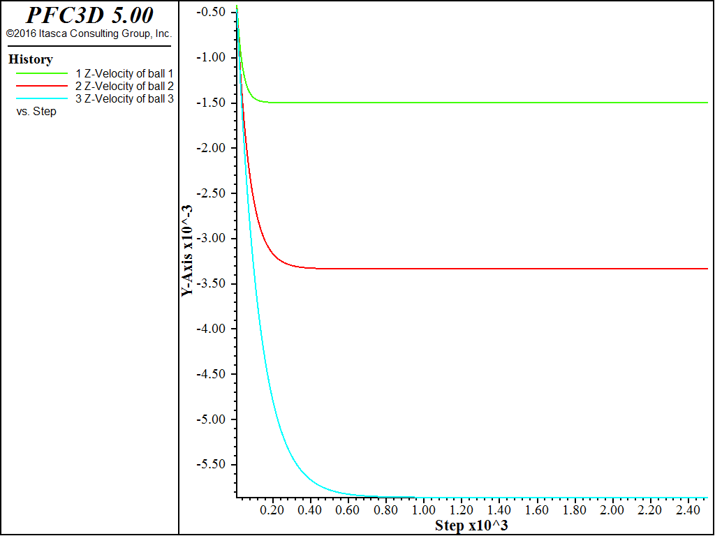
Figure 1: Histories of ball velocities (\(z\)-component)

[Batchelor1967]

G.K. Batchelor, An Introduction to Fluid Dynamics. Cambridge University Press, Cambridge. 1967.