Block with a Slipping Crack under Cyclic Loading
Problem Statement
Note
The project file for this example may be viewed/run in 3DEC.[1] The main data files used are shown at the end of this example.
The problem concerns an elastic block with an inclined, internal, closed crack subjected to a uniaxial load cycle. (Note: This section was prepared under Contract No. NRC-02-88-005 with the Center for Nuclear Waste Regulatory Analysis (CNWRA).)
The problem shown in Figure 1 consists of a three-dimensional block with an inclined, closed crack extending along the entire length of the block in the \(z\)-direction. Axial displacement, applied on top of the model, is gradually increased and then decreased until the original position of the model is restored. The resulting load causes inelastic slip on the crack. The stress-displacement relation for the load cycle, as shown in Figure 2, is composed of three distinct components (Olsson 1982):
a loading segment (OA) which features both elastic deformation and slip along the crack;
an initial unloading segment (AB), where the crack does not slip; and
a final unloading segment (BO), again with both elastic deformation and slip.
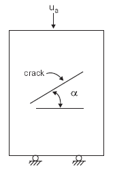
Figure 1: Three-dimensional block with embedded planar crack.
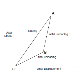
Figure 2: Stress-displacement relation for an elastic block with embedded crack subjected to uniaxial load cycle (see Olsson 1982).
The following problem conditions are prescribed for the evaluation. A single inclined crack is embedded in an elastic medium. The physical properties of the medium are:
elastic modulus (\(E'\)): 88.9 GPa
Poisson’s ratio (\(\nu '\)): 0.26
height (\(H\)): 2 m
width (\(W\)): 1 m
length (\(B\)) 1 m
The properties of the crack are:
joint normal stiffness (\(K_n\)): 220 GPa /m
joint shear stiffness (\(K_s\)): 220 GPa /m
joint friction angle (\(\phi\)): 16°
joint inclination (\(\alpha\)): 45°
slipping portion of crack (\(\ell\)): 0.54 m
Conceptual Model
The conceptual model (presented by Brady et al. (1985)) considers the deformational response of a single crack embedded in an elastic solid. For convenience, in the 3DEC analysis, the three-dimensional representation of the model illustrated in Figure 3 has a discontinuity of length \(L\) (of which only the central portion of length \(\ell\) is allowed to slip), \(B\) is the depth of the block, and the crack in the \(y\)-direction.
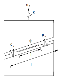
Figure 3: Conceptual model of elastic block containing embedded crack (see Brady et al. 1985).
The equivalent axial elastic stiffness of the specimen, including the through-going discontinuity, is given as
where \(W B E' / H\) is the uniaxial elastic stiffness of the solid, and the two remaining terms are contributions from the normal (\(K_n\)) and shear (\(K_s\)) spring stiffness of the joint.
The stiffnesses for the three slopes are given by:
The modulus of elasticity, \(E'\), and Poisson’s ratio, (\(\nu\)), from Equation (1) are the plane-stress parameters; the corresponding plane-strain parameters are \(E\) and \(\nu\). The relation between the plane-stress and plane-strain elastic constants is given by:
and
It should be noted that the conceptual model presented by Brady et al. (1985) assumes plane-stress conditions.
3DEC Model
Assumptions
It was assumed that the block material in which the crack is embedded is linearly elastic, homogeneous and isotropic. The crack plane is inclined at an angle of 45° with respect to the \(xz\)-plane, and runs across the block in the \(z\)-direction. The central strip of the discontinuity along the \(z\)-direction is allowed to slip. The ends of the discontinuity are prevented from slipping by setting the frictional resistance to a high value over these regions.
Model Geometry and Zones
The elastic block with a planar crack was modeled with elastic, deformable blocks, as shown in Figure 4. All of the joints except the discontinuity were “joined” in order to model a continuous elastic medium. Each block was discretized into tetrahedral zones.
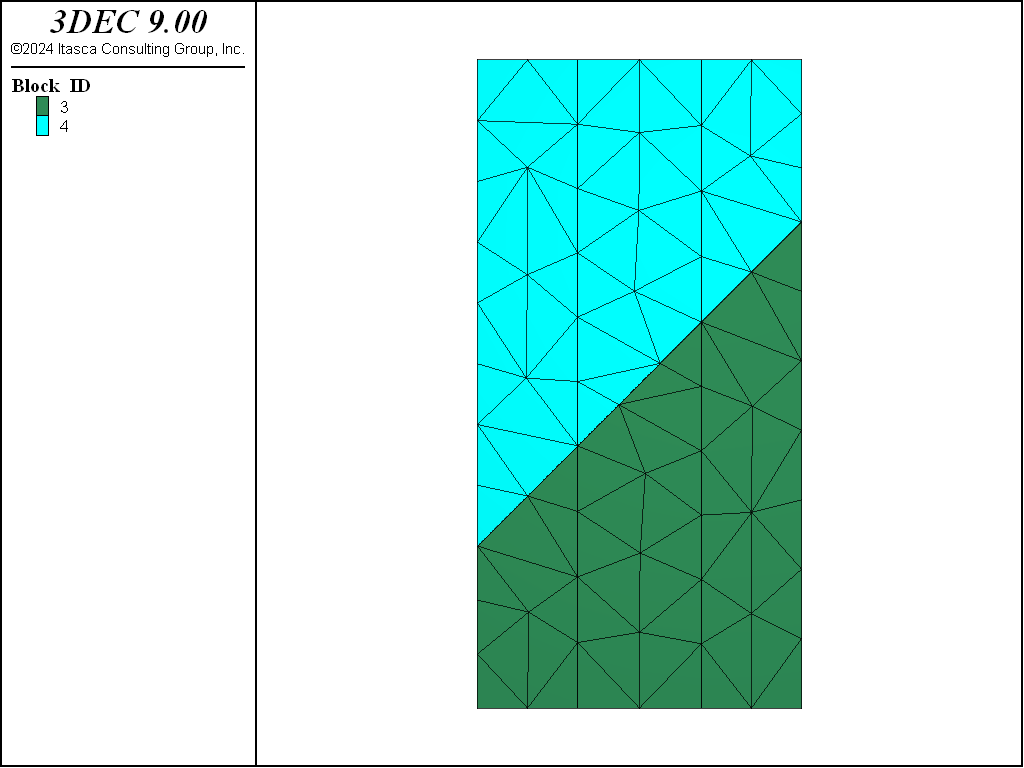
Figure 4: Block model of the three-dimensional specimen with planar crack.
Joint Parameters
The standard Coulomb slip model was used for joints. The Coulomb model is a linear, elastic, perfectly plastic constitutive relation and corresponds to the concepts used in developing the expressions for three stiffnesses in the conceptual model (Equations (1) through (4)). The joint properties are given in the table below.
Normal stiffness, stiffness-normal |
220 GPa/m |
Shear stiffness, stiffness-shear |
220 GPa/m |
Friction, friction |
16^{circ} |
Boundary Conditions
The bottom boundary along the \(xy\)-plane was fixed at \(y\) = 0.
A plane-strain condition was simulated by restricting the displacement in the \(z\)-direction. This was done by setting the velocity boundary conditions to zero along the \(xy\)-plane at \(z\) = 0 and \(z\) = 1.0.
A plane-stress condition was simulated by keeping all four vertical boundaries free.
Loading
A complete load cycle in uniaxial compression was performed by applying a velocity boundary condition to the top of the model. The magnitude of the velocity was controlled by a servo executed using a FISH function (see “SLIP.FIS”). The loading and unloading sequence was also implemented and controlled using a FISH function.
Results
Vertical stress versus vertical displacement curves (obtained using the analytic solution and calculated by 3DEC) are shown in Figure 5 and Figure 6. Figure 5 compares the analytic solution with the results obtained by 3DEC for plane-strain conditions; Figure 6 compares the analytic solution with the results obtained by 3DEC for plane-stress conditions. (A FISH function was used to calculate the average displacements and average stress at the top of the model. The analytical results were also calculated using a FISH function.)
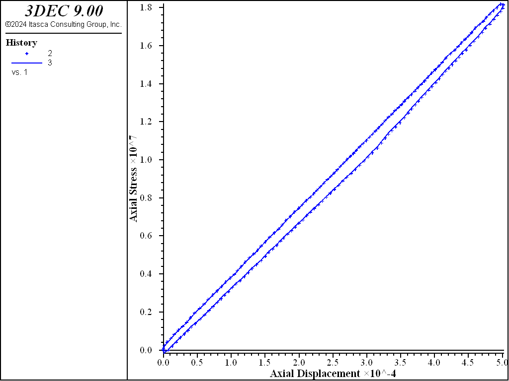
Figure 5: Plane-strain conditions — axial stress versus axial displacement for the problem involving cyclic loading for a block with a slipping crack modeled with Coulomb friction law.
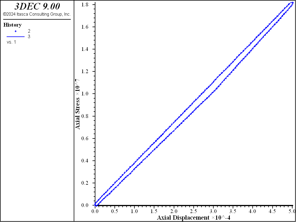
Figure 6: Plane-stress conditions — axial stress versus axial displacement for the problem involving cyclic loading for a block with a slipping crack modeled with Coulomb friction law.
Discussion
This simple conceptual model captures the essential features of a loading cycle of an elastic body with a slipping crack. The complete loading cycle is accompanied by three distinct slopes, representing loading with slip, initial unloading without slip and unloading with slip. When modeling both plane-stress and plane-strain conditions, it can be seen that the results from the 3DEC analysis with the Coulomb joint model agree well with the conceptual model.
However, it was observed that as the length of the slipping crack increases with respect to the width of the specimen, the results from the 3DEC analysis do not agree as well. This is expected, because the conceptual model assumes uniform distribution of normal stress on the crack and the elastic extensions. In practice, stress concentrations (particularly joint normal stress) become more significant as the length of the slipping crack increases.
References
Brady, B. H. G., M. L. Cramer and R. D. Hart. “Preliminary Analysis of a Loading Test on a Large Basalt Block (Tech. Note),” Int. J. Rock Mech. Min. Sci. & Geomech. Abstr., 22, 345-348 (1985).
Olsson, W. A. “Experiments on a Slipping Crack,” Geophys. Res. Letters, 9(8), 797-800 (1982).
Data Files
slip3d.dat
;==============================================================
; verification test -- slipping crack
;
;   3dec modeling of block with slipping crack under cyclic load
;   Joint Model: Coulomb Slip Model
;   elastic blocks
;==============================================================
;
;
model new
fish automatic-create off
model large-strain on

fish define params
  global W_ = 1.0      ; width
  global B_ = 1.0      ; length
  global H_ = 2.0      ; height
  global E_ = 88.9e9   ; Young's modulus (plane stress)
  global poiss_ = 0.26 ; Poisson's ratio (plane stress)
  global alpha_ = 45   ; joint dip angle
  global l_ = 0.54     ; slipping length of crack
  global fric_ = 16    ; jopint friction angle
  global jkn_ = 220e9  ; joint normal stiffness
  global jks_ = 220e9  ; joint shear stiffness

  global E_planestrain = E_*(1.0+2.0*poiss_)/(1.0+poiss_)^2
  global poiss_planestrain = poiss_/(1.0+poiss_)

  global crack_xmin = 0.5*W_ - math.cos(alpha_*math.degrad)*0.5*l_
  global crack_xmax = 0.5*W_ + math.cos(alpha_*math.degrad)*0.5*l_
  global crack_zmin = 0.5*H_ - math.sin(alpha_*math.degrad)*0.5*l_
  global crack_zmax = 0.5*H_ + math.sin(alpha_*math.degrad)*0.5*l_

  global vel_          ; initial loading velocity
  global displim_      ; displacement limit
  global unbal_limit = 1000  ; unbalanced force limit used in servo control
end
[params]
;
block create brick 0,[W_] 0,[B_] 0,[H_]
block cut joint-set dip [-alpha_] dip-direction 90 origin 0.0,0.0,0.5
block cut joint-set dip  90 dip-direction 90 origin [crack_xmin],0.0,0.0 join
block cut joint-set dip  90 dip-direction 90 origin [crack_xmax],0.0,0.0 join
block zone generate edgelength 0.2
;
; crack extension - no slip
block zone cmodel elastic
block zone property density 2850 young [E_planestrain] ...
                    poisson [poiss_planestrain]

block contact jmodel mohr
block contact property stiffness-normal [jkn_] ...
                       stiffness-shear [jks_]  ...
                       friction 89.0           ...
                       tension 100

; crack properties
block contact property stiffness-normal [jkn_] stiffness-shear [jkn_] ...
                       friction [fric_] ...
                       range position-x [crack_xmin],[crack_xmax] ...
                             position-z [crack_zmin-0.001],[crack_zmax+0.001]
block contact material-table default property stiffness-normal [jkn_] ...
                                              stiffness-shear [jkn_]  ...
                                              friction [fric_]

block insitu stress -0.1 -0.1 -0.1 0 0 0

; set up list of gridpoints on top boundary
program call 'slip.fis'
[_boulist]

block mechanical damping global
history interval 100
fish history disp_avg
fish history stress_avg
fish history astress
fish history vel_
model history mechanical unbalanced-maximum

history name '1' label 'Axial Displacement'
history name '2' label '3DEC'
history name '3' label 'Analytic'
;
model save 'slip3d-ini'
;==============================================================
;   verification part I
;   plane strain simulation
;==============================================================
;
; boundary conditions
;
block gridpoint apply velocity-z 0 range position-z [H_]
block gridpoint apply velocity-z 0 range position-z 0.0
block gridpoint apply velocity-y 0 range position-y 0.0
block gridpoint apply velocity-y 0 range position-y [B_]

[vel_ = -1e-5]
[displim_ = 5e-4]

; load over input number of steps
[_load(100)]

; unload
[vel_ = 1e-6]
[displim_ = 0]
[_load(100)]

;
model save 'slip3d-planestrain'
;==============================================================
;   verification part II
;   plane stress simulation
;==============================================================
;
model restore 'slip3d-ini'

block zone property young [E_] poisson [poiss_]
;
;
; boundary conditions
;
block gridpoint apply velocity-z 0 range position-z [H_]
block gridpoint apply velocity-z 0 range position-z 0.0
;
[vel_ = -1e-5]
[displim_ = 5e-4]

; load over input number of steps
[_load(100)]

; unload
[vel_ = 1e-6]
[displim_ = 0]
[_load(100)]
;
model save 'slip3d-planestress'
;
program return
slip.fis
;==================================================
;
; derivation of analytic solution for moduli
;
;==================================================
fish define _analytic
  local cos_al_ = math.cos(alpha_*math.degrad)
  local sin_al_ = math.sin(alpha_*math.degrad)
  local Length_ = W_/cos_al_
  local invk_ = H_/(W_*B_*E_)+cos_al_*cos_al_/(jkn_*Length_*B_)
  invk_ = invk_+sin_al_*sin_al_/(jks_*Length_*B_)
  local k_ = 1./invk_
  global slopeAB_ = k_
  local den_     = jks_*B_*(Length_-l_)*math.cos(fric_*math.degrad)
  local den1_    = k_*sin_al_*math.sin((alpha_-fric_)*math.degrad)/den_
  local den2_    = k_*sin_al_*math.sin((alpha_+fric_)*math.degrad)/den_
  global slopeOA_ = k_/(1.+den1_)
  global slopeBO_ = k_/(1.+den2_)
  global dispmax_ = 0.0
end
[_analytic]
;==================================================
;
; sets a list of boundary grid points at which the
; load is applied
;
;==================================================
fish define _boulist
  global points = map
  loop foreach local igp_ block.gp.list
    local z_ = block.gp.pos.z(igp_)
    if math.abs(H_-z_) < 0.01*H_ then
        points(map.size(points)) = igp_ ; Store in map, arbitrary unique index
    end_if
  end_loop
end
;
;=======================================================
;
; calculation of average stress and displacement on the
; top of the model; and calculation of analytic relation
; between stress and displacements
;
;=======================================================
fish define stress_avg
  local xc_ = 0.5*W_
  local yc_ = 0.5*B_
  local zc_ = H_
  local igp_ = block.gp.near(xc_,yc_,zc_)

  global disp_avg = -block.gp.disp.z(igp_)

  if vel_ < 0. then
    global astress = slopeOA_*disp_avg
  else
    local ua_      = dispmax_
    local ub_      = dispmax_*(slopeOA_-slopeAB_)/(slopeBO_-slopeAB_)
    if disp_avg > ub_ then
      astress = dispmax_*slopeOA_ - (dispmax_-disp_avg)*slopeAB_
    else
      astress = disp_avg*slopeBO_
    end_if
  end_if
  local stress_ = 0.0
  loop foreach local gp points
      stress_ = stress_ - block.gp.force.reaction.z(gp)
  end_loop
  stress_avg = stress_/(W_*B_)
;  loop foreach local zp block.zone.list
;    stress_ = stress_ - block.zone.stress.zz(zp)
;  end_loop
;  stress_avg = stress_ / float(block.numzone)
end
;
;==================================================
;
; function which controls cycling
;
;==================================================
fish define _load(nstep_)
  local sign_ = vel_/math.abs(vel_)
  loop while 1 > 0
    command
      model cycle [nstep_]
    end_command
    if sign_*disp_avg < sign_*displim_
      dispmax_ = disp_avg
      exit
    end_if
  end_loop
end
;==================================================
;
; servo mechanism which controls the loading on the
; model
;
;==================================================
fish define _servo
  while_stepping
  if block.unbal > unbal_limit then
    vel_ = 0.98*vel_
    loop foreach local gp points
      block.gp.vel.app.z(gp) = vel_
    end_loop
  endif
  if block.unbal < 0.8*unbal_limit then
    vel_ = 1.02*vel_
    loop foreach gp points
      block.gp.vel.app.z(gp) = vel_
    end_loop
  endif
end
Endnote
| Was this helpful? ... | Itasca Software © 2024, Itasca | Updated: Nov 12, 2025 |
