Hydraulic Fracture
Note
The project file for this example may be viewed/run in 3DEC.[1] The main data files used are shown at the end of this example.
Problem Statement
The propagation of a vertical hydraulic fracture constrained within a 20 m thick horizontal layer is analyzed. Fluid with a 1 cP (10−3 pa × s) viscosity is injected through the vertical borehole at the total rate of 2 × 10⁻³ m3/s, uniformly distributed over the thickness of the layer. The fracture propagates in a homogeneous, isotropic elastic medium with a Young’s modulus of 10 GPa, and a Poisson’s ratio of 0.2.
Warning
This problem takes a long time to run. When running this verification problem, allow 12-24 hours (depending on computer speed) for the calculation to complete.
Analytical Solution
The evolution of the pressures and fracture widths in this problem can be approximated by the PKN solution (Perkins and Kern 1961) under the following assumptions:
linear elastic fracture mechanics (LEFM) theory is applicable;
the pressure gradient in the direction of fracture propagation is created by the flow resistance in a narrow elliptically shaped channel;
the fracture has a fixed height, \(H\), independent of the distance from the wellbore, \(x\);
in any vertical elliptical cross-section perpendicular to the direction of propagation, the fluid pressure, \(p\), is constant (i.e., no vertical pressure drop);
at the tip of the fracture \(p_{net}\) = 0 (i.e., the fracturing fluid pressure is equal to confining stress, \(\sigma_c\), at the crack tip); and
plane-strain deformation occurs in the vertical cross sections – each identical vertical section acts independently (only valid if \(L\) >> \(H\)).
The geometry of the PKN model and the important model variables are illustrated in Figure 1.
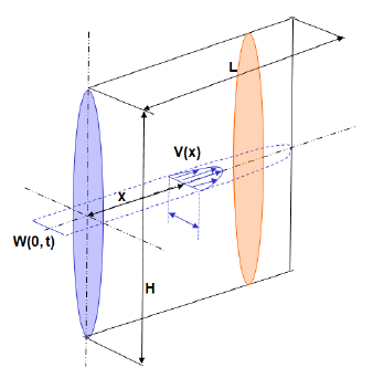
Figure 1: Geometry of the PKN model.
According to the PKN solution (Perkins and Kern 1961), the net pressure, \(p_{net}\), can be approximated using the following expression:
while the expression for the width (aperture) in the middle of the fracture is
where \(E\) is the Young’s modulus, \(\nu\) is the Poisson’s ratio, \(q\) is the injection rate, \(\mu\) is the viscosity of the injected fluid, and \(L\) and \(H\) are the length and height of the fracture, respectively, as illustrated in Figure 1.
3DEC Model
The 3DEC model uses the symmetry of the problem and represents one (upper) half of the fracture only. The trace of the fracture is predefined in 3DEC by the vertical contact plane, which is initially joined together but allowed to open (fracture) only within the constant-height layer during the simulation as dictated by stress changes induced by the injected fluid. (The vertical contact plane is not allowed to fracture outside the predefined layer.) The fracture plane is the only discontinuity within the model. The PKN solution is for a fracture in an infinite elastic medium. Because the 3DEC model size must be finite, it is selected to be sufficiently large compared to the size of the fracture (i.e., fracture height, \(H\), and the fracture length, \(L\), achieved during the simulation) such that the deformation of the fracture is not affected by the model size, but also considering the effects on the model runtime (because too large of a model would require long simulation time). The model geometry is illustrated in Figure 2. The discretization of the model, shown in Figure 3, illustrates the graded mesh with the finest discretization of 1 m zone size near the fracture and the coarsest discretization of 4 m zone size away from the fracture, along the far-field boundaries.
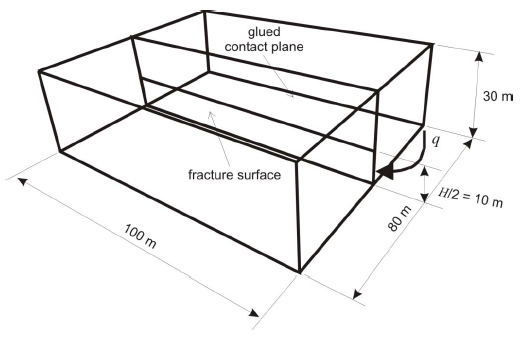
Figure 2: Geometry of the 3DEC PKN model.
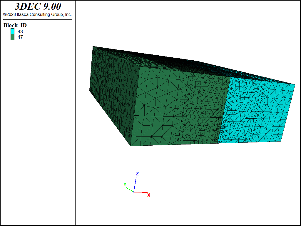
Figure 3: Discretization of the 3DEC PKN model.
“Roller” boundary conditions were applied on all outside boundaries of the mechanical model. The fluid was injected at the specified rate along the vertical edge of the fracture surface as indicated in Figure 2.
Results and Discussion
After 368 s of injection, the fracture was approximately 75 m long, which was considered sufficient to satisfy the assumption (i.e., \(L/H\) = 75/20 = 3.75 >> 1) used in derivation of the PKN solution. At the state after 368 s of injection, the 3DEC results are compared with the PKN solution. The state of the 3DEC model is illustrated by the contour plots of displacements, fluid pressure, and apertures shown in Figures 4 through 6, respectively. The fluid pressure contours in Figure 5 illustrate that there is no pressure gradient in the vertical direction, except near the injection point and the fracture tip, as approximated by the PKN solution.
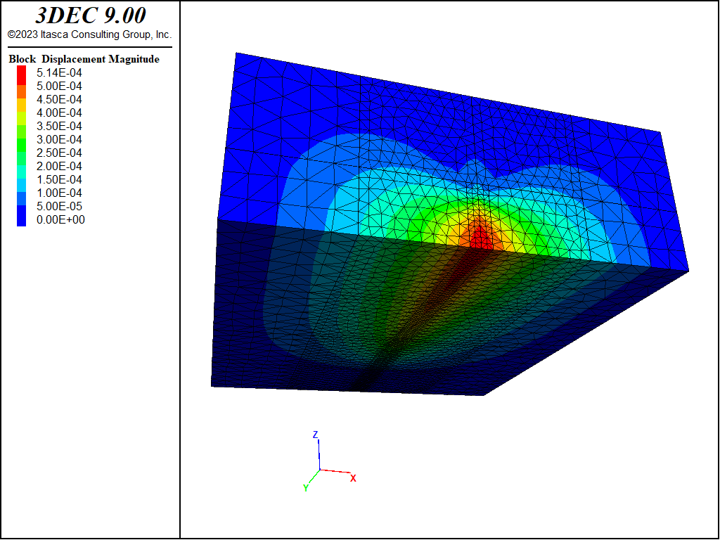
Figure 4: Displacement magnitude contours (m) predicted in the 3DEC PKN model.
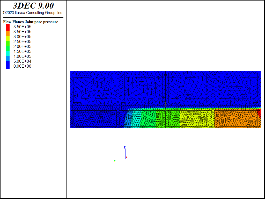
Figure 5: Fracture pressure contours (Pa) in the 3DEC PKN model.
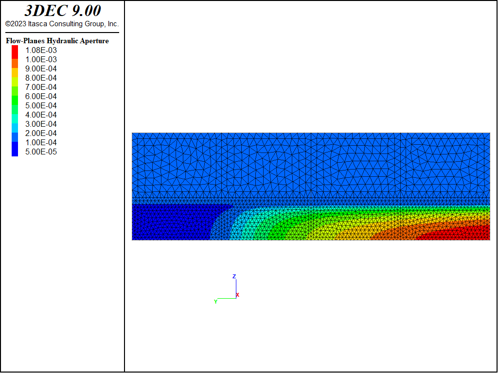
Figure 6: Fracture width (aperture) contours (m) in the 3DEC PKN model.
The net pressure profile, as calculated in 3DEC, is shown in Figure 7. The fracture widths (apertures) predicted in 3DEC and using the PKN solution are compared in Figure 8. Overall, the 3DEC predictions are in reasonably good agreement with the PKN solution. The match of the maximum widths is particularly good near the injection point. As expected, the discrepancy is greatest near the fracture tip. 3DEC uses constant strain zones of uniform size along the entire fracture. Thus, the approximation in the 3DEC model of the stress singularity and strain gradients near the fracture tip is relatively poor. The second reason for the poor match near the fracture tip is that the minimum fracture aperture in the 3DEC model cannot be smaller than the user-specified residual aperture. The motivation for this limit is to prevent model instability when the flow equations become singular as the aperture decreases to zero. Typically, the residual aperture is selected to be a small value compared to prevailing apertures in the model. In these simulations, the residual aperture was assumed to be 50 \(\mu m\). Comparisons of the maximum net pressure and fracture widths as calculated using 3DEC and the PKN solution are provided in Table 1. The match is good, with an error less than 7%.
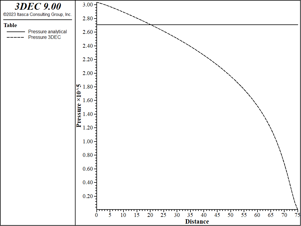
Figure 7: Profile of the net pressure along the fracture predicted in the 3DEC PKN model.
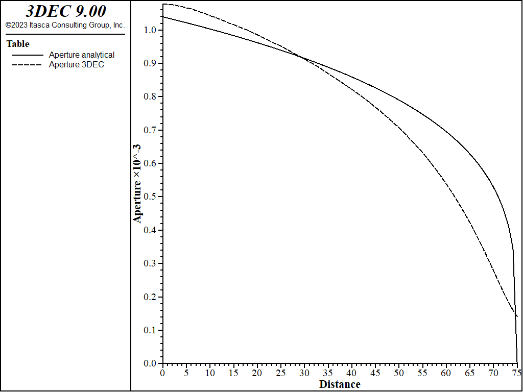
Figure 8: Profile of the maximum widths (aperture) predicted by the PKN analytical solution and 3DEC.
PKN |
3DEC |
Error (%) |
|
|---|---|---|---|
w(0) (mm) |
1.039 × 10⁻³ |
1.037 × 10⁻³ |
0.2 |
p(0) (Pa) |
2.71 × 10⁵ |
2.89 × 10⁵ |
6.6 |
Reference
Perkins, T., and L. Kern. “Widths of hydraulic fractures,” J. Pet. Tech., 222, pp. 937-949 (1961).
Data Files
pkn.dat
; file: pkn.dat
; example of hydraulic fracturing

model new
model random 10000
;
fish automatic-create off
model configure fluid
model large-strain off

fish define geometry

  global fractureLength = 10.0

  local modelWidth = 8.*fractureLength
  local modelHeight = 3.*fractureLength
  local modelLength = 10.*fractureLength

  global x1 = -0.5*modelWidth
  global x12 = -0.25*modelWidth
  global x2 = 0.
  global x21 = -0.2*fractureLength
  global x22 =  0.2*fractureLength
  global x23 = 0.25*modelWidth
  global x3 = 0.5*modelWidth
  global y1 = 0.
  global yh1 = 0.25*modelLength
  global yh = 0.5*modelLength
  global yh2 = 0.75*modelLength
  global y2 = modelLength
  global z1 = 0.
  global z2 = fractureLength
  global z21 = z2+0.2*fractureLength
  global z3 = modelHeight
  global edge1 = 0.1*fractureLength
  global edge2 = 0.2*fractureLength
  global edge3 = 0.4*fractureLength
  global edgelength = edge1
  global z1l = z1-0.2*edge
  global z2l = z2-0.2*edge
  global z2h = z2+0.2*edge
  global z3h = z3+0.2*edge
  global x2l = x2-0.2*edge
  global x2h = x2+0.2*edge
  global y1l = y1-0.2*edge
  global y1h = y1+0.2*edge
end
[geometry]
block create brick [x1] [x3] [y1] [y2] [z1] [z3]
block cut joint-set dip 0 dip-direction 0 origin [x2] [y1] [z21]
block cut joint-set dip 90 dip-direction 90 origin [x2] [y1] [z1]
block cut joint-set dip 90 dip-direction 0 origin [x2] [yh] [z1]
block cut joint-set dip 90 dip-direction 0 origin [x2] [yh1] [z1]
block cut joint-set dip 90 dip-direction 0 origin [x2] [yh2] [z1]
block cut joint-set dip 90 dip-direction 90 origin [x12] [y1] [z1]
block cut joint-set dip 90 dip-direction 90 origin [x23] [y1] [z1]
block hide range plane dip 0 dip-direction 0 origin [x2] [y1] [z21] above
block cut joint-set dip 90 dip-direction 90 origin [x21] [y1] [z1]
block cut joint-set dip 90 dip-direction 90 origin [x22] [y1] [z1]
block hide range plane dip 90 dip-direction 90 origin [x21] [y1] [z1] below
block hide range plane dip 90 dip-direction 90 origin [x22] [y1] [z1] above
block cut joint-set dip 0 dip-direction 0 origin [x2] [y1] [z2]
block hide off
;
block hide range plane dip 90 dip-direction 90 origin [x2] [y1] [z2] above
block join on
block hide off
block hide range plane dip 90 dip-direction 90 origin [x2] [y1] [z2] below
block join on
block hide off
block zone generate edgelength [edge1] ...
  range position-x [x21] [x22] position-z [z1] [z21]
block zone generate edgelength [edge2] range position-x [x12] [x23]
block zone generate edgelength [edge3]
;
model save 'pkn-zoned'

model restore 'pkn-zoned'
;
block gridpoint apply velocity-x 0. range position-x [x1]
block gridpoint apply velocity-x 0. range position-x [x3]
block gridpoint apply velocity-y 0. range position-y [y1]
block gridpoint apply velocity-y 0. range position-y [y2]
block gridpoint apply velocity-z 0. range position-z [z1]
block gridpoint apply velocity-z 0. range position-z [z3]
;
[global pois_ = 0.2]
[global E_ = 1e10]
block zone cmodel assign elastic
block zone property density 2600. young [E_] poiss [pois_]

block contact jmodel assign mohr
block contact property stiffness-normal 1e9 ...
                       stiffness-shear 1e9 ...
                       cohesion 1e4 ...
                       tension 1e4
flowplane vertex property aperture-initial 0.5e-4 ...
                          aperture-minimum 0.5e-4 ...
                          aperture-maximum 1e-2
block contact property stiffness-normal 1e10 ...
                       stiffness-shear 1e10 ...
                       tension 1e30 ...
                       cohesion 1e30 ...
                       range position-z [z2l] [z3h]
flowplane vertex property aperture-initial 1e-4 ...
                       aperture-minimum 1e-4 ...
                       aperture-maximum 1e-4 ...
                       range position-z [z2l] [z3h]

block fluid crack-flow on
;
[global visc_=1e-3]
[global inj_=2e-3]
block fluid property bulk 2e7
block fluid property density 1000.
block fluid property viscosity [visc_]

; injecting into half of fracture, so discharge is injection rate/length/2
flowplane edgelength apply discharge [inj_/fractureLength/2.0] ...
                     range position-x [x2l] [x2h] ...
                           position-y [y1l] [y1h] ...
                           position-z [z1l] [z2h]
;
model mechanical active on
model fluid active on
;model fluid follower on
;model fluid substep 10
model mechanical follower on
model mechanical substep 1
model solve fluid time-total 368
model save 'pkn'
;
program call 'PKN_verify'
;
program return
pkn_verify.dat
; file pkn_verify.dat
;
;
[global frac_length = 75.0]
[global frac_height = 20.0]
;
; analytical solution forigin aperture and pressure
; along y axis
; aperture stored in table '1'
; pressure stored in table '3'
;
fish define _analytical
  ; pressure from PKN solution
  local numerator_ = 16.0*visc_*inj_*E_*E_*E_*frac_length
  local denominator_ = (1.0-pois_*pois_)^3*math.pi*frac_height^4
  local pressure_ = math.sqrt(math.sqrt(numerator_/denominator_))
  loop foreach local gp_ block.gp.list
      local z_ = block.gp.pos.z(gp_)
      if z_ < 0.01
        local y_ = block.gp.pos.y(gp_)
        if y_ < 75.1
          ; aperture eqn from PKN solution
          local aperture_=3*((visc_*inj_*(1-pois_^2)*(frac_length-y_))/E_)^0.25
          table(1,y_) = aperture_
          table(3,y_) = pressure_
        endif
      endif
  end_loop
end
;
; 3DEC aperture and pressure along y axis
; aperture stored in table '2'
; pressure stored in table '4'
;
fish define _3DEC
  loop foreach local fpe_ flowplane.vertex.list
      local coord_global = flowplane.vertex.pos(fpe_)
      if comp.z(coord_global) < 0.01
        local y_ = comp.y(coord_global)
        if y_ < 75.1
          local aperture_ = flowplane.vertex.aperture.hydraulic(fpe_)
          table(2,y_) = aperture_
          local knot_ = flowplane.vertex.knot(fpe_)
          local pressure_ = flowknot.pp(knot_)
          table(4,y_) = pressure_
        endif
      endif
  end_loop
end
;
[_analytical]
[_3DEC]

table '1' label 'Aperture analytical'
table '2' label 'Aperture 3DEC'
table '3' label 'Pressure analytical'
table '4' label 'Pressure 3DEC'
Endnote
| Was this helpful? ... | Itasca Software © 2024, Itasca | Updated: Nov 12, 2025 |
