Tutorial: Quick Start (3DEC)
This tutorial will address the fundamental steps when using 3DEC for the first time. It will help new users become comfortable with beginning new projects and developing a simple block model. A walk-through guide of a simple wedge failure example will be completed. Interactive controls using both the mouse and script commands input in the 3DEC console will be explained and illustrated.
Topics:
rigid blocks
joints
histories
GUI and plot manipulation
Commands: BLOCK CREATE, BLOCK DELETE, BLOCK FIX, BLOCK GROUP, BLOCK HIDE, BLOCK CUT, BLOCK PROPERTY, MODEL CYCLE, MODEL GRAVITY, MODEL SAVE
FISH: none
- Files: “Users_Guide/getting_started/simple_wedge/simple_wedge.prj”
“Users_Guide/getting_started/simple_wedge/simple_wedge.dat”
Project
After starting 3DEC, you will be shown a dialog box with information about the version you are using. At the bottom of the dialog are several startup options related to projects. A project is simply a way to bundle together data files, FISH files, plots, etc. related to a problem being solved with 3DEC. Select “New Project …” from the prompt.
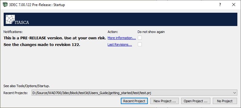
Figure 1: Project file-loading options during startup
A save prompt will now appear. Click on the My Projects directory on the left, and save the new project as “getting_started.prj”. When you install 3DEC, a directory called My Projects is created for you in Documents/Itasca/3dec700. This is a useful place to store your own projects.
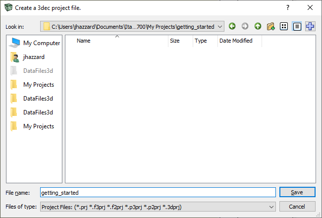
Figure 2: Project file save dialog
The commands used to complete this tutorial will be saved in a data (٭.dat) file. To create a new data file, select or press Ctrl+N. Save the new data file as “simple_wedge.dat” in the same folder as the project file (“getting_started.prj”).
Layout
The 3DEC GUI (graphical user interface) contains display panels for data files, plots, the command console and project files. The layout of the panes in the 3DEC GUI can be customized to suit any user’s preference. There are several predefined layout options found under the “Layout” menu, including “Horizontal,” “Vertical,” “Single,” “Wide” and “Project” options. A 3DEC layout can also be saved and restored by setting up the preferred layout using the mouse and dragging different panes into place. Once the panes are in place, click “Layout” and select “Save layout….” A prompt will appear and request a save location for the layout file. This location is necessary when restoring saved layout preferences.
Choose and your screen should appear as shown.
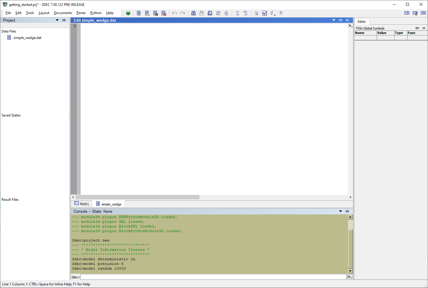
Figure 3: 3DEC “Wide” layout
The newly created data file is listed under “Data Files,” on the left. The blank data file itself fills the main pane. The command console is at the bottom. When the data file is shown, a table of global FISH symbols is whon in the right. If a plot is shown, plot controls are on the right (select the Plot01 tab to see this).
Creating a Model
Now we can begin inputting commands to create the model. Commands can either by entered into the file and then executed later, or they can be entered one by one in the console at the bottom. It is recommended that commands be entered into the file because this will save them and allow you to easily run the same set of commands multiple times.
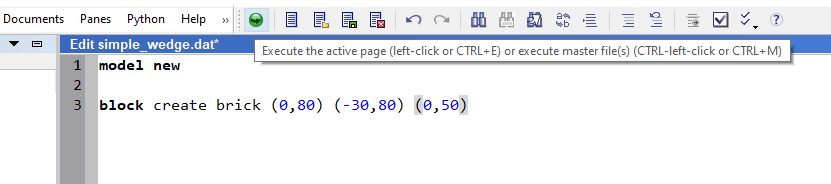
The following commands will clear previous model information, create the initial block and specify the block size. We specify a single polyhedral block using the block create brick command.
model new
block create brick (0,80) (-30,80) (0,50)
This will create a block with the dimensions 80 × 110 × 50. At any time, you can press Ctrl + spacebar to see keywords following a command. The keywords shown can be clicked and new keywords will then appear. In this way a command can be built up with minimal typing or memorizing of keywords. At any time it is also possible to press F1 to bring up the relevant section of the manual related to the command or keyword.
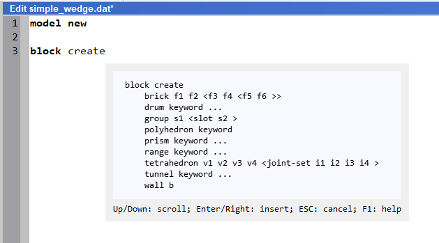
Figure 4: An example of context sensitive help in 3DEC.
Execute the file by clicking on the green execute button.
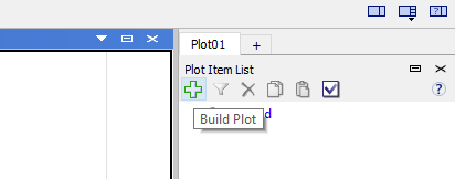
To view the plot, select the Plot01 tab below the editor window. The plot controls will now appear on the right side. Select the Build Plot button as shown.
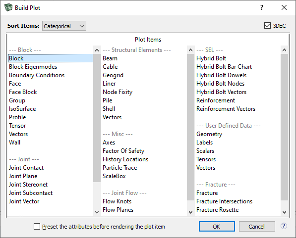
You will now see a ist of all possible plot items. Select Block and click OK.
The single block should now appear in the plot window. The default view of the model is oriented parallel to the \(xz\)-plane. Try holding down the right mouse button and moving the mouse, to rotate the plot. The figure below illustrates a rotated view of the block.
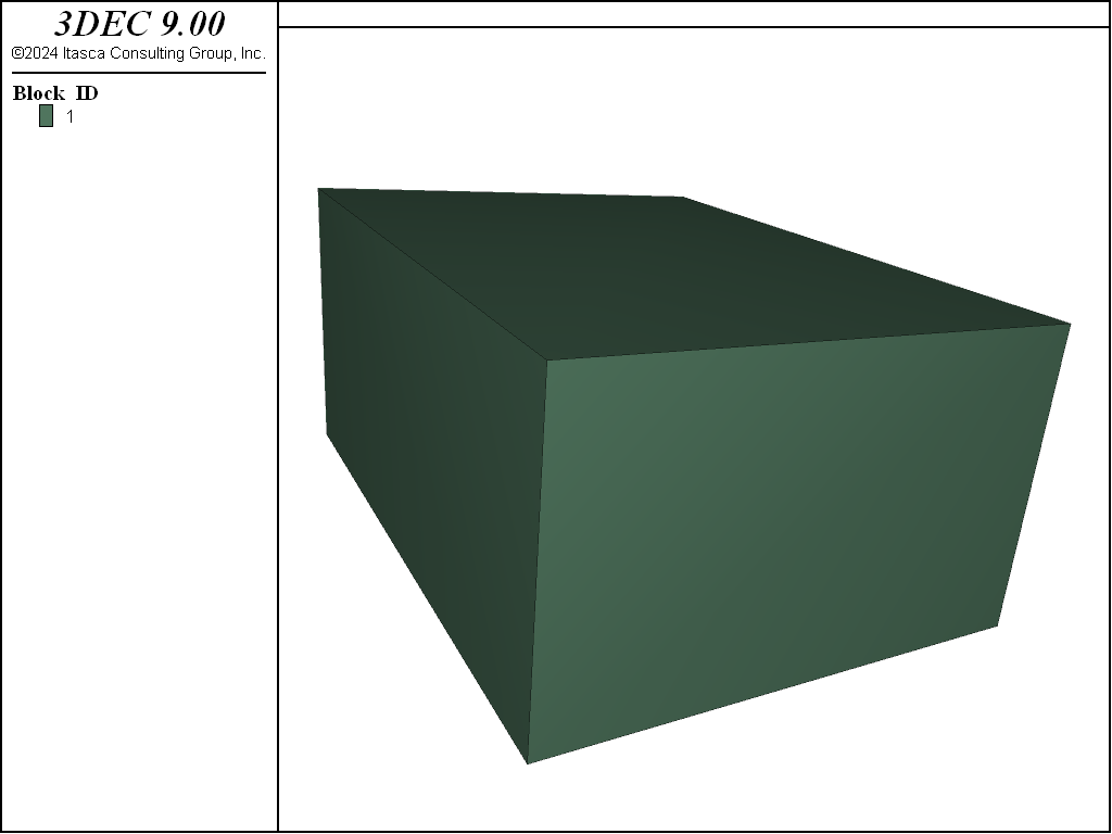
Figure 8: 3DEC block plot
You can rename the plot by right-clicking on the Plot01 tab and selecting . Change the plot name to Blocks.
Manipulating the view: Press and hold the right mouse button and drag the mouse across the plot
to rotate the model; press and hold right-click + left-click to pan; zoom in and out using the scroll wheel. Press Ctrl + R to reset the view back to the xz plane.
For more detailed instructions on view manipulation, right-click on the plot and select .
Creating the Joint Sets
Joints are introduced to the model by using the block cut joint-set command. Joints can represent actual rock joints, or they can be used as “construction” cuts to create specific geometries. For this example, a series of joint sets are implemented in order to create the slope and wedge. We begin by cutting the joint horizontally in two locations using the keywords dip, dip-direction and origin. CAUTION: If no keywords are used, these properties will default to values of 0.
Click on the “simple_wedge” tab to go back to the data file and add the following commands.
block cut joint-set dip 90 dip-direction 180 origin 0,0,0
block cut joint-set dip 90 dip-direction 180 origin 0,50,0
The dip direction is degrees clockwise from North (\(y\)). The block is cut into three (3) sections along the \(y\)-axis. The middle block is assigned to a group named “inner block” using a RANGE command to specify a range in \(y\)-coordinates for the block centroids. The other blocks are called “outer blocks” to define the blocks that act as boundaries.
block group 'inner block' range pos-y 0 50
block group 'outer blocks' range group 'inner block' not
Execute the file. Click on the “Blocks” tab to see the block plot. You will now see three blocks of different colors. In the control panel on the right, click on the “Block Block” item. In “Attributes,” under “Label”, select .
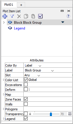
Figure 9: Block plot item attributes dialog
The block plot will now look like this:
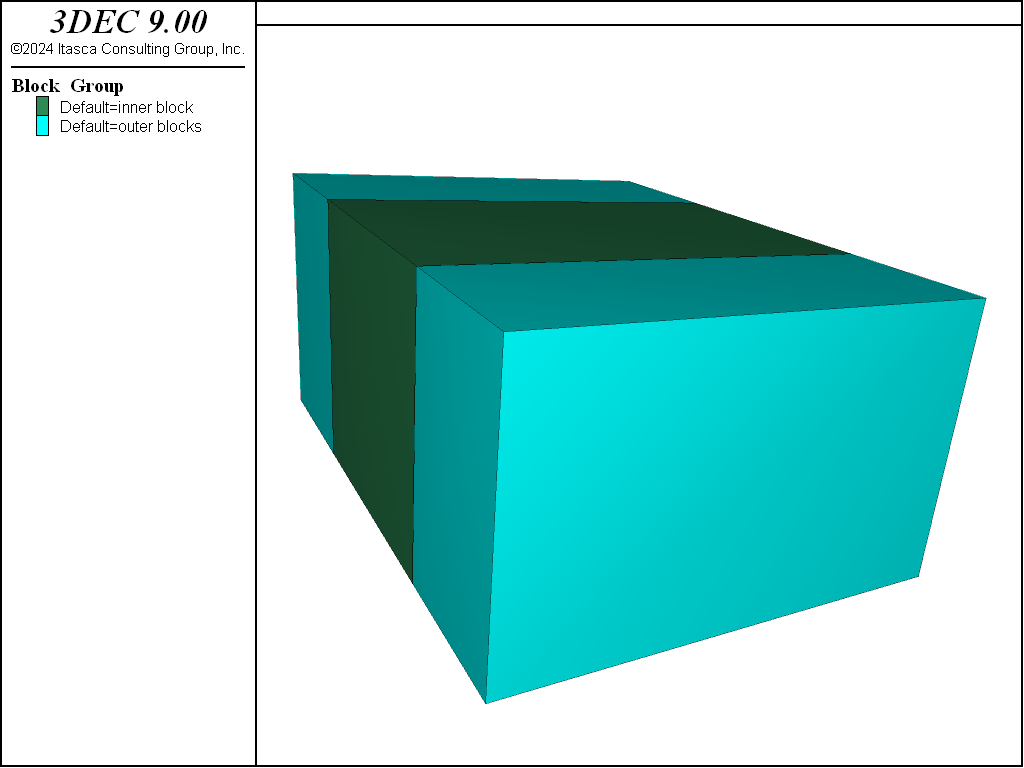
Figure 10: Original block split into three blocks
Additional joint sets are introduced into the model and create the sliding planes for the future wedge in both the horizontal and vertical directions.
First, hide the outer blocks. A block hide command is used to do this. Hidden blocks are not cut by \(block cut\) commands.
Two (2) shallow-dipping fracture planes are created, and then five (5) equally spaced high angle foliation planes are made.
block hide range group 'outer blocks'
block cut joint-set dip 2.5 dip-direction 235 origin 30,0,12.5
block cut joint-set dip 2.5 dip-direction 315 origin 35,0,30
block cut joint-set dip 76 dip-direction 270 spacing 4 num 5 origin 38,0,12.5
The use of the spacing keyword specifies an average spacing distance between joints. The num keyword defines the number of joints in the set. Execute the file and click on the “Blocks” plot tab. Change the “Label” back to “Block”. The model should look similar to the figure below.
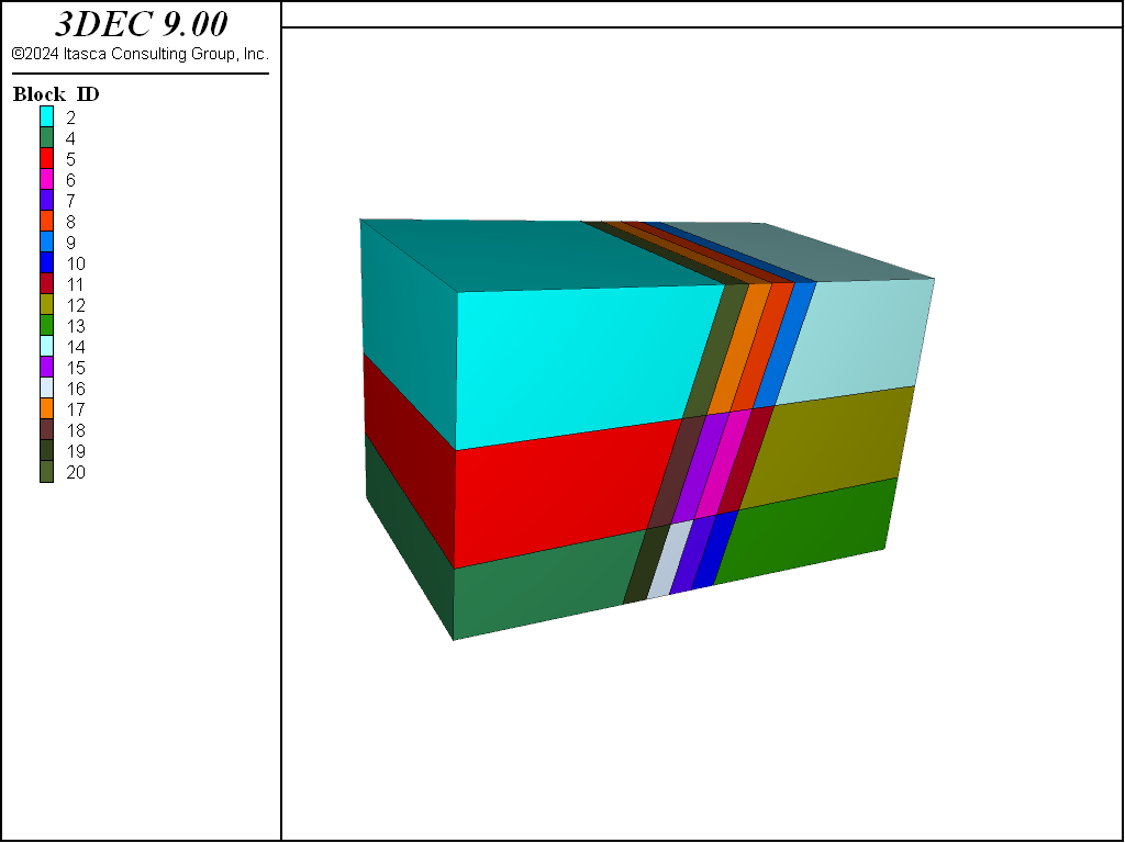
Figure 11: Joint planes added
We now hide the slope blocks and create a horizontal joint plane which will make up the base of the slope excavation.
block hide range pos-x 30,80 pos-y 0,50 pos-z 0,50
block cut joint-set dip 0 dip-direction 0 origin 0,0,10
block hide range pos-z 0,10
block group 'excavate'
We assign the blocks within the excavate region to a group called “excavate.”
Creating the Wedge Feature
Finally, we create the joint planes that define the wedge in the slope using the following commands:
block hide off
block hide range group 'outer blocks'
block hide range pos-z 0,10
block hide range pos-x 55,80
block hide range pos-x 0,30
block cut joint-set dip 70 dip-direction 200 origin 0,35,0
block cut joint-set dip 60 dip-direction 330 origin 50,15,50
Executing the file at this point will show the blocks with the high angle foliations and the planes that define the wedge as shown below.
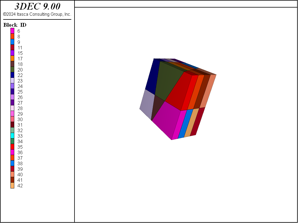
Figure 12: Wedge blocks added
Boundary Conditions
Next, the boundary blocks are immobilized. Using the block fix command and specifying the necessary range will freeze each block’s centroid velocity at its current value. In this case, the centroid velocity is currently zero. This will prevent any movement, thus creating boundary conditions. If you fix a block that is already moving, the block will continue to move at that current velocity. The base of the model and the blocks behind the foliations are fixed in place. The outer blocks are also fixed. The “excavate” group is deleted from the model. The outer blocks are left hidden for plotting purposes.
block hide off
block fix range pos-z 0 10
block fix range pos-x 55 80
block fix range group 'outer blocks'
block hide range group 'outer blocks'
block delete range group 'excavate'
Go back to the “Blocks” plot. Add axes to the plot by selecting the “Build Plot” button (+) and choosing .
The axes can be resized by left-clicking and dragging the edges of the item. They can be moved by left-clicking and dragging the middle of the item. The plot should now look similar to the plot below.
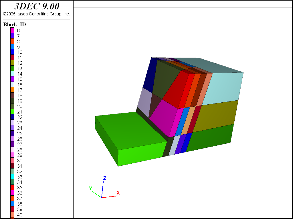
Figure 13: Completed model view
Gravity
The model gravity command assigns a gravitational acceleration in the negative z-direction. In this example, we specify a value of 10 m/sec2. The \(x\) and \(y\) components are 0.
model gravity 0 0 -10
Material Properties
Note
٭Mass density of the block material, not the unit weight, is assigned.
The material properties are assigned to the blocks and joints. It is first necessary to show the hidden blocks so that they are assigned properties too.
In this example, the mass density٭ of all blocks is specified to be 2,000 units (kg/m3, in this case). Blocks are assumed to be rigid; block deformability is neglected.
block hide off
block property density 2000
Joint properties are assigned next. Before joint properties can be assigned, subcontacts need to be generated with the command block contact generate-subcontacts. This command triangulates the block surfaces and adds subcontacts at the triangle vertices. It is necessary to have multiple subcontacts per contact to resist rotation.
Note that this step is not necessary if you are using deformable blocks and you have given the block zone generate command to create zones. In this case, the face triangulation matches the zone faces.
All joints have the same normal and shear stiffness, equal to 1.0 × 10^9 units (Pa/m, in this case; see Joint Properties for a discussion on how to choose joint stiffness values). The true joints assigned a friction angle of 89º (for now), and the joints between the inner and outer blocks are assigned a friction angle of 0º.
The “boundary” joints are identified with a group name so we can identify them again later.
block contact generate-subcontacts
block contact prop stiffness-norm=1e9 stiffness-shear=1e9 friction=89
block contact group 'boundary' range orientation dip 90 dip-dir 180
block contact prop fric=0.0 range group 'boundary'
If running the model in large strain, it is also necessary to define the properties for any new contacts that may form when blocks are sliding. This is done with the following command:
block contact material-table default prop stiffness-norm=1e9 stiffness-shear=1e9 fric=0
Note
It is possible in 3DEC to abbreviate the commands, as long as there are enough characters that they can be uniquely identified. For example, property can be abbreviated as prop.
It is possible to specify different contact properties for different blocks that come into contact, hence the need for a “material table”. In this case, we can assume that all new contacts are frictionless.
Note that different constitutive models are available for joints. In this example, a simple Mohr-Coulomb model is used (the default).
Solution
The problem is ready to be solved. It is often helpful to judge material behavior by observing the motion of specified points in the rock mass. In this problem, we monitor the \(z\)-velocity of a vertex nearest the point \(x\) = 40, \(y\) = 40, \(z\) = 50. In this example, we need to be careful to select a point on the wedge and not the corresponding point in the host rock. For this reason we will first hide the blocks on one side of the joint as shown before taking the history.
block hide range plane dip 70 dip-direction 200 origin 0,35,0 below
block history vel-z position (40,40,50)
Following execution of this command, the program returns information about the selected monitoring point.
We then show the blocks again, hide the outer blocks:
block hide off
block hide range group 'outer blocks'
Finally, we bring the model to equilibrium with the following commands. Before cycling, we need to indicate if we are running in large or small strain using the model large-strain command. We can then use the model solve command to reach equilibrium. Note that the blocks won’t slide because we have initialy specified a high friction angle.
model large-strain on
model solve
Execute the file by clicking the green execute button at the top. During execution, the current cycle count, the calculation time, the maximum out-of-balance force (Unbalanced force is defined in Reaching Equilibrium), and the clock time are printed on the screen every 10 cycles. Inspection of these values indicates that equilibrium has been achieved (unbalanced force approaches zero).
Create a new plot called “Vel His” by selecting and entering the name at the prompt. In the control panel, select the “Build Plot” button (+) and then choose , and a blank history chart will appear. Next, under the “Attributes” tab, add the “Z-velocity” history by clicking the blue “+” symbol. Note that each history is assigned an ID when it is created. Since we only have one history, it is assigned an ID of 1. The blue “+” symbol allows you to add the history of ID 1 to the plot.
Change the label for the \(y\)-axis by selecting and entering “vertical velocity.”
The plot should look like this:
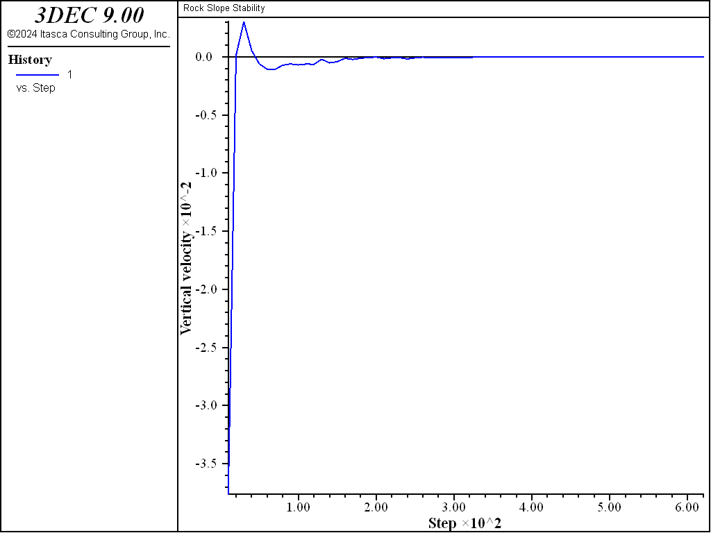
Figure 14: History of vertical velocity during equilibrium cycling
Plot Image Files
After the model has been brought to equilibrium, creating an image file of a plot of the initial state may be useful. A plot title can be provided using the model title command and including a string afterwards:
model title 'Rock Slope Stability'
The title will be saved but not displayed to the plot. In order to display the title on the plot, click the “View Settings” button above the plot items (it looks like a check mark in a box). Then check the “Job Title” box in the resulting dialog.
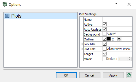
Figure 15: Display setting dialog
The title will appear at the top of the plot, above the history. The properties of the title such as size, font, style (bold, italic, bold italic) and color can be modified in the Options dialog.
The plot can then be exported as several different file types. Navigate under , or simply right-click on the plot and select . A plot and file name must be specified. It is also possible to export the history data as comma-separated values in a text file by right-clicking and selecting .
Save Initial State
It is good practice to save the initial state of the model so that it can be restarted at any time (for example, to perform parameter studies). We save the current state to a file called “slope-initial.sav” by typing
model save 'slope-initial'
The file name extension .sav is automatically added if no extension is given.
Reduce Joint Friction and Solve
The behavior of the slope can be studied by reducing the friction angle of the joints. We reduce the friction angle to 6º using the following commands (either add to the file and re-execute, or simply type the command into the console at the bottom of the 3DEC GUI):
block contact prop fric=6.0 range group 'boundary' not
The next step is to continue the calculations with the reduced friction for an additional 2000 cycles. We don’t want to use model solve since it is unlikely that the model will reach equilibrium. The failure can be seen on the “Blocks” plot. For plotting purposes, turn on the job title by going to “View Settings” in the control panel (the check-mark in a box) and checking the “Job Title” option. This will add the job title specified previously. To add a title specific to this plot, check on the “Plot Title” option and enter some text (e.g., “Wedge Failure”).
To watch the failure progress, type the following command in the console at the bottom of the screen and press :
model cycle 2000
Upon executing the problem, the block plot will illustrate the wedge failure caused by the reduction in the friction angle. The failure mode combines rotational failure along the foliation planes and rotational failure of the wedge. The wedge failure dominates the failure, as shown by the block plot. The rotational mechanism contributes to the collapse.
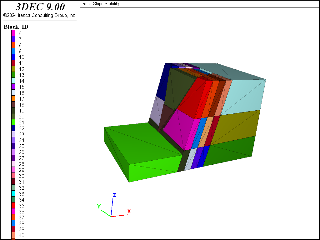
Figure 16: Wedge sliding down
Cross Section
A vertical cross-section plot taken through the model will demonstrate the rotational mechanism. Click and name the plot “Cross Section”. From the list of plot items, select . By default, the vectors will show displacement, but this can be changed with the Type attribute. Under the “Attributes”, toggle the “By-Magnitude” option on.
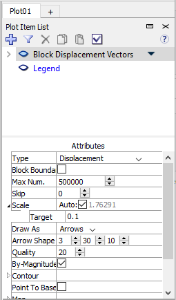
Figure 17: Displacement vectors plot-item attribute dialog
Add blocks to the plot. The fill is toggled off by clicking on the box in the “Attributes”.
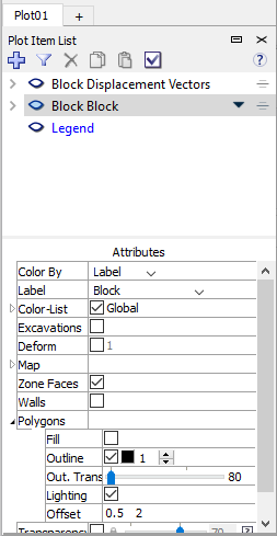
Figure 18: Block plot-item attribute dialog
Finally, a cutting plane is required to create the cross section. This is done by clicking on the “Cutting Tool” under the “Block Block” plot item. By default, the plane will cut perpendicular to the current view, half-way through the model. So in this case, the plane is normal to the \(y\)-axis (0,1,0) and the origin is at \(y\) = 25.
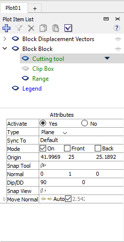
Figure 19: Cut plane plot-item attributes dialog
Also turn on the cut plane for the Block Displacement Vectors plot item. The resulting cross section displaying the displacement vectors:
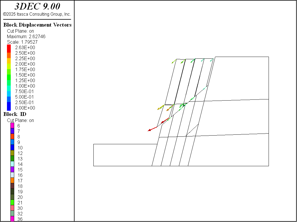
Figure 20: Cross section on cut plane showing blocks and displacement vectors
Conclusion
This concludes the getting started tutorial. Save the project by clicking . You will be asked if you also want to save the model state. Click “Yes” and save the model as ‘slope-final’. From this point forward, you may wish to try other various 3DEC features in an attempt to stabilize the slope. You can restart from the initial state by entering
model restore 'slope-initial'
There are structural elements that can be incorporated and are described in Structural Elements.
| Was this helpful? ... | Itasca Software © 2024, Itasca | Updated: Nov 12, 2025 |
