Joint Properties

Choosing Joint Properties

Joint properties are conventionally derived from laboratory testing (e.g., triaxial and direct shear tests). These tests can produce physical properties for joint friction angle, cohesion, dilation angle and tensile strength, as well as joint normal and shear stiffnesses. The joint cohesion and friction angle correspond to the parameters in the Coulomb strength criterion.

Values for normal and shear stiffnesses for rock joints typically can range from roughly 10 to 100 MPa/m for joints with soft clay in-filling, to over 100 GPa/m for tight joints in granite and basalt. Published data on stiffness properties for rock joints are limited; summaries of data can be found in Kulhawy (1975), Rosso (1976) and Bandis et al. (1983).

Approximate stiffness values can be back-calculated from information on the deformability and joint structure in the jointed rock mass and the deformability of the intact rock. If the jointed rock mass is assumed to have the same deformational response as an equivalent elastic continuum, then relations between jointed rock properties and equivalent continuum properties can be derived.

For uniaxial loading of rock containing a single set of uniformly spaced joints oriented normal to the direction of loading, the following relation applies:

(1)\[\begin{split}\frac{1}{E_m}=\frac{1}{E_r}+\frac{1}{k_ns} \\ \\\end{split}\]

or

\[k_n=\frac{E_mE_r}{s(E_r-E_m)}\]

where:	\(E_m\)	=   rock mass Young’s modulus;
	\(E_r\)	=   intact rock Young’s modulus;
	\(k_n\)	=   joint normal stiffness; and
	\(s\)	=   joint spacing.

A similar expression can be derived for joint shear stiffness:

(2)\[k_s=\frac{G_mG_r}{s(G_r-G_M)}\]

where:	\(G_m\)	=   rock mass shear modulus;
	\(G_r\)	=   intact rock shear modulus; and
	\(k_s\)	=   joint shear stiffness.

The equivalent continuum assumption, when extended to three orthogonal joint sets, produces the following relations:

(3)\[\begin{split}\begin{align} E_i&=\left(\frac{1}{E_r}+\frac{1}{s_ik_{ni}}\right)^{-1} &(i=1, 2, 3) \\ \\ G_{ij}&=\left(\frac{1}{G_r}+\frac{1}{s_ik_{si}}+\frac{1}{s_jk_{sj}}\right)^{-1} &(i,j=1,2,3) \end{align}\end{split}\]

Several expressions have been derived for two- and three-dimensional characterizations and multiple joint sets. References for these derivations can be found in Singh (1973), Gerrard (1982(a) and (b)) and Fossum (1985).

There is a limit to the maximum joint stiffnesses that are reasonable to use in a 3DEC model. If the physical normal and shear stiffnesses are less than ten times the equivalent stiffness of adjacent zones, then there is no problem with using physical values. If the ratio is more than ten, the solution time will be significantly longer than for the case in which the ratio is limited to ten, without much change in the behavior of the system. Serious consideration should be given to reducing supplied values of normal and shear stiffnesses to improve solution efficiency usinbg the following relation:

(4)\[k_n < 10\left[max\left[\frac{K+4/3G}{∆z_{min}}\right]\right]\]

where \(K\) and \(G\) are the bulk and shear moduli of the block material and \(\Delta z_{min}\) is the smallest dimension of the zone adjoining the joint in the normal direction.

There may also be problems with block interpenetration if the normal stiffness, kn, is very low. A rough estimate should be made of the joint normal displacement that would result from the application of typical stresses in the system (\(u = \sigma/k_n\)). This displacement should be small compared to a typical zone size. If it is greater than, say, 10% of an adjacent zone size, then either there is an error in one of the numbers or the stiffness should be increased.

Published strength properties are more readily available for joints than for stiffness properties. Summaries can be found, for example, in Jaeger and Cook (1969), Kulhawy (1975) and Barton (1976). Friction angles can vary from less than 10º for smooth joints in weak rock (such as tuff), to over 50º for rough joints in hard rock (such as granite). Joint cohesion can range from zero cohesion to values approaching the compressive strength of the surrounding rock.

It is important to recognize that joint properties measured in the laboratory typically are not representative of those for real joints in the field. Scale dependence of joint properties is a major question in rock mechanics. Often, the only way to guide the choice of appropriate parameters is by comparison to similar joint properties derived from field tests; however, field test observations are extremely limited. Some results are reported by Kulhawy (1975).

Joint Persistence

Often joints are faults are not 100% persistent. Rock bridges or asperities prevent continuous sliding. Since 3DEC blocks cannot be partially cut, the easiest way to

Contact Material Table

In large strain mode (model large-strain on), default contact constitutive models and properties must be defined for potential new contacts. Joint constiutive models and properties can be assigned to existing contacts with the block contact jmodel assign command and block contact property command respectively. For contacts that have not yet formed, the constitutive model and properties will be taken from the contact material table. The contact material table is a table of ranges and the associated joint consitutive models and properties.

An entry is added to the table with the block contact material-table command. The add keyword allows the user to specify an entry consisting of a range, a joint model and properties. The default keyword sets the joint model and properties for all new contacts not defined by another entry in the table. If large-strain is on, the default properties must be assigned. If not given, the default constitutive model is assumed to be mohr-coulomb.

A simple example is shown below. A slope is created composed of three different material types, defined by three different group names as shown in Figure 1. A single block slides down the slope. Different contact properties are assigned when different block groups come into contact as shown in the data file below. In this example, the default friction angle is 30^o, but the friction angle for contact between the sliding block and blocks with group base2 is 40^o. Since the slope angle is greater than 30^o and less than 40^o, the block slides initially, but then stops wne it overlaps the middle block with the group name base2. A plot of the x-velocity of the sliding block is shown in Figure 2

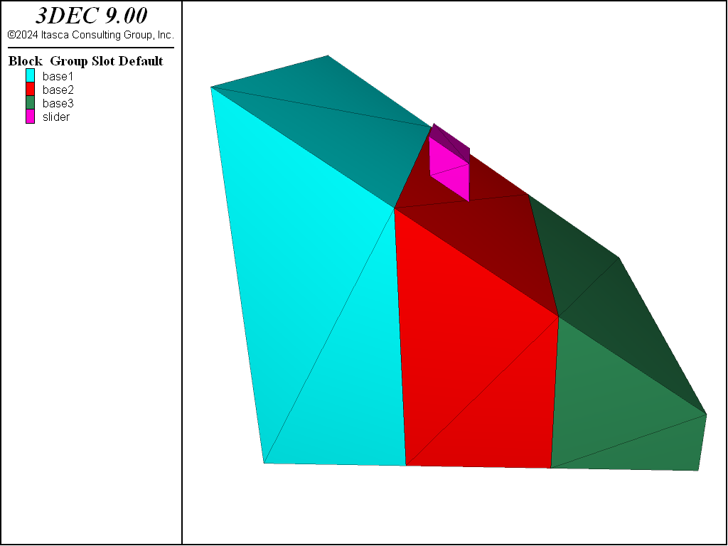
Figure 1: Model of the sliding block.

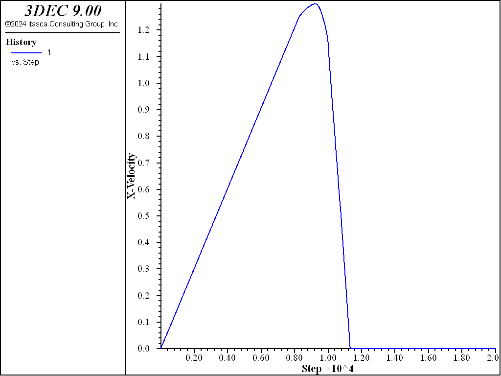
Figure 2: X-velocity history of the sliding block.

The full data file is below.

; test assiging of joint properties using the material table

model new

; create slope
block create brick -10 10
block cut joint-set dip 35 dip-direction 90
block delete range position-z 0 10

; divide into three sections
block densify segments 3 1 1
block group 'base1' range position-x -10 -3
block group 'base2' range position-x -3 3
block group 'base3' range position-x 3 10

; create block to slide down the slope
[tan35 = math.tan(35*math.degrad)]
block create prism face-1 -10,-2,[10*tan35] ...
                          -10,-2,[2+10*tan35] ...
                          -8,-2,[2+8*tan35] ...
                          -8,-2,[8*tan35] ...
                    face-2 -10,2,[10*tan35] ...
                          -10,2,[2+10*tan35] ...
                          -8,2,[2+8*tan35] ...
                          -8,2,[8*tan35] ...
                    group 'slider'

block fix range group 'base1' or 'base2' or 'base3'

block property density 2000

block contact material-table default property ...
  stiffness-normal 1e9 stiffness-shear 1e9 friction 30

; assign different properties to new contacts 
;   that form between 'slider' and 'base2'
block contact material-table add jmodel mohr property ...
  stiffness-normal 1e9 stiffness-shear 1e9 friction 40 ...
  range group-intersection 'slider' 'base2'
  
model gravity 0 0 -10

model large-strain on

block history velocity-x position -9 0 [1+10*tan35]

model cycle 20000

Joint Persistence

Often a joint or fault is not fully persistent - meaning that there are rock bridges or asperities separating sliding sections. Since 3DEC blocks cannot be partially cut, the easiest way to account for non persistent faults is to zone them first (or generate subcontacts) and then assign different properties to different parts of the fault.

This is similar to the way in which DFN fractures are dealt with (see Discrete Fracture Networks), except in this case there are no fractures that can be used to define bonded and unbonded sections of the fault.

The block contact persistence command allows for the creation of contiguous patches on a fault that can be considered rock bridges or asperities. The user specifies a perisistence (between 0 and 1), a length for the rock bridges, and a group name. Patches of subcontacts will then be assigned the specified group name so that the user can easily change the properties (or constitutive model) of these subcontacts. An example is shown below. Note that the persistence is not exactly as specified. In general, the resulting persistence is within a few percent of that specified.

model new

block create brick -10 10
block densify segments 5 join
block cut joint-set dip 30 dip-direction 90
block zone generate edgelength 0.5

block contact persistence 0.7 length 2 bridge-group 'bridge' 

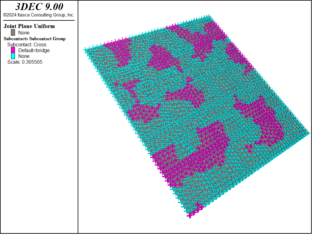
Figure 3: Joint plane showing subcontact groups. Rock bridges are pink. The specified persistence is 0.7. The true persistence is calculated to be 0.688.

If the persistence is less than 50%, it may be preferable to think of the sliding portions of the fault to be circular patches and the remainder of the fault to be considered “rock bridge”. In this case, you can use the same command, but for persistence enter one minus the true persistence, and for bridge-group give a group name for the active fault. An example is shown below. Note that a different random seed is used to produce a different pattern of patches.

model new
model random 10010

block create brick -10 10
block densify segments 5 join
block cut joint-set dip 30 dip-direction 90
block zone generate edgelength 0.5

block contact group 'bonded'

; actual persistence is 0.3
block contact persistence 0.7 length 2 bridge-group 'sliding_fault' 

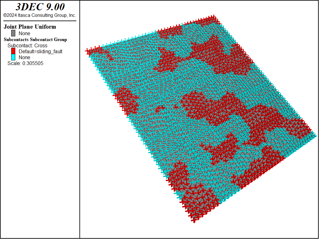
Figure 4: Joint plane showing subcontact groups. Section of sliding joint are red. The specified “persistence” is 0.7. The calculated “persistence” is 0.64. Note that in this case, the patches are considered to be sliding joints, so the persistence is really 0.36.